Note
This tutorial was generated from an IPython notebook that can be downloaded here.
theano version: 1.0.4
pymc3 version: 3.6
exoplanet version: 0.1.5
Fitting TESS FFIs¶
This tutorial is nearly identical to the tess tutorial with added support for the TESS full frame images using tesscut.
First, we query the TESS input catalog for the coordinates and properties of this source:
import numpy as np
from astroquery.mast import Catalogs

ticid = 49899799
tic = Catalogs.query_object("TIC {0}".format(ticid), radius=0.2, catalog="TIC")
star = tic[np.argmin(tic["dstArcSec"])]

tic_mass = float(star["mass"]), float(star["e_mass"])
tic_radius = float(star["rad"]), float(star["e_rad"])
Then we download the data from tesscut. This is similar to what we did in the tess tutorial, but we need to do some background subtraction because the pipeline doesn’t seem to do too well for the official TESS FFIs.
from io import BytesIO
from zipfile import ZipFile
from astropy.io import fits
from astropy.utils.data import download_file
# Download the cutout
url = "https://mast.stsci.edu/tesscut/api/v0.1/astrocut?ra={0[ra]}&dec={0[dec]}&y=15&x=15&units=px§or=All".format(star)
fn = download_file(url, cache=True)
with ZipFile(fn, "r") as f:
with fits.open(BytesIO(f.read(f.namelist()[0]))) as hdus:
tpf = hdus[1].data
tpf_hdr = hdus[1].header
texp = tpf_hdr["FRAMETIM"] * tpf_hdr["NUM_FRM"]
texp /= 60.0 * 60.0 * 24.0
time = tpf["TIME"]
flux = tpf["FLUX"]
m = np.any(np.isfinite(flux), axis=(1, 2)) & (tpf["QUALITY"] == 0)
ref_time = 0.5 * (np.min(time[m])+np.max(time[m]))
time = np.ascontiguousarray(time[m] - ref_time, dtype=np.float64)
flux = np.ascontiguousarray(flux[m], dtype=np.float64)
# Compute the median image
mean_img = np.median(flux, axis=0)
# Sort the pixels by median brightness
order = np.argsort(mean_img.flatten())[::-1]
# Choose a mask for the background
bkg_mask = np.zeros_like(mean_img, dtype=bool)
bkg_mask[np.unravel_index(order[-100:], mean_img.shape)] = True
flux -= np.median(flux[:, bkg_mask], axis=-1)[:, None, None]
Everything below this line is the same as the tess tutorial.
import matplotlib.pyplot as plt
from scipy.signal import savgol_filter
# A function to estimate the windowed scatter in a lightcurve
def estimate_scatter_with_mask(mask):
f = np.sum(flux[:, mask], axis=-1)
smooth = savgol_filter(f, 1001, polyorder=5)
return 1e6 * np.sqrt(np.median((f / smooth - 1)**2))
# Loop over pixels ordered by brightness and add them one-by-one
# to the aperture
masks, scatters = [], []
for i in range(1, 100):
msk = np.zeros_like(mean_img, dtype=bool)
msk[np.unravel_index(order[:i], mean_img.shape)] = True
scatter = estimate_scatter_with_mask(msk)
masks.append(msk)
scatters.append(scatter)
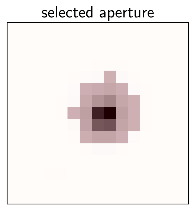
# Choose the aperture that minimizes the scatter
pix_mask = masks[np.argmin(scatters)]
# Plot the selected aperture
plt.imshow(mean_img.T, cmap="gray_r")
plt.imshow(pix_mask.T, cmap="Reds", alpha=0.3)
plt.title("selected aperture")
plt.xticks([])
plt.yticks([]);
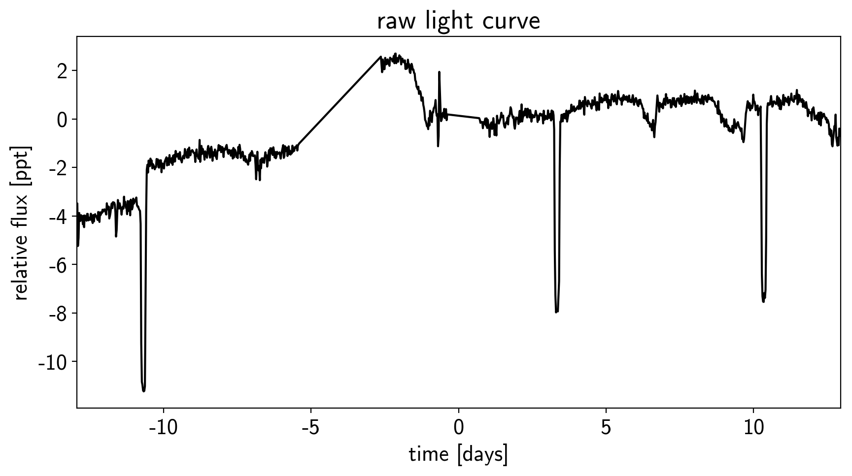
plt.figure(figsize=(10, 5))
sap_flux = np.sum(flux[:, pix_mask], axis=-1)
sap_flux = (sap_flux / np.median(sap_flux) - 1) * 1e3
plt.plot(time, sap_flux, "k")
plt.xlabel("time [days]")
plt.ylabel("relative flux [ppt]")
plt.title("raw light curve")
plt.xlim(time.min(), time.max());
# Build the first order PLD basis
X_pld = np.reshape(flux[:, pix_mask], (len(flux), -1))
X_pld = X_pld / np.sum(flux[:, pix_mask], axis=-1)[:, None]
# Build the second order PLD basis and run PCA to reduce the number of dimensions
X2_pld = np.reshape(X_pld[:, None, :] * X_pld[:, :, None], (len(flux), -1))
U, _, _ = np.linalg.svd(X2_pld, full_matrices=False)
X2_pld = U[:, :X_pld.shape[1]]
# Construct the design matrix and fit for the PLD model
X_pld = np.concatenate((np.ones((len(flux), 1)), X_pld, X2_pld), axis=-1)
XTX = np.dot(X_pld.T, X_pld)
w_pld = np.linalg.solve(XTX, np.dot(X_pld.T, sap_flux))
pld_flux = np.dot(X_pld, w_pld)
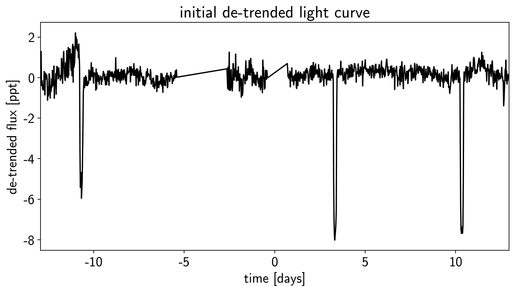
# Plot the de-trended light curve
plt.figure(figsize=(10, 5))
plt.plot(time, sap_flux-pld_flux, "k")
plt.xlabel("time [days]")
plt.ylabel("de-trended flux [ppt]")
plt.title("initial de-trended light curve")
plt.xlim(time.min(), time.max());
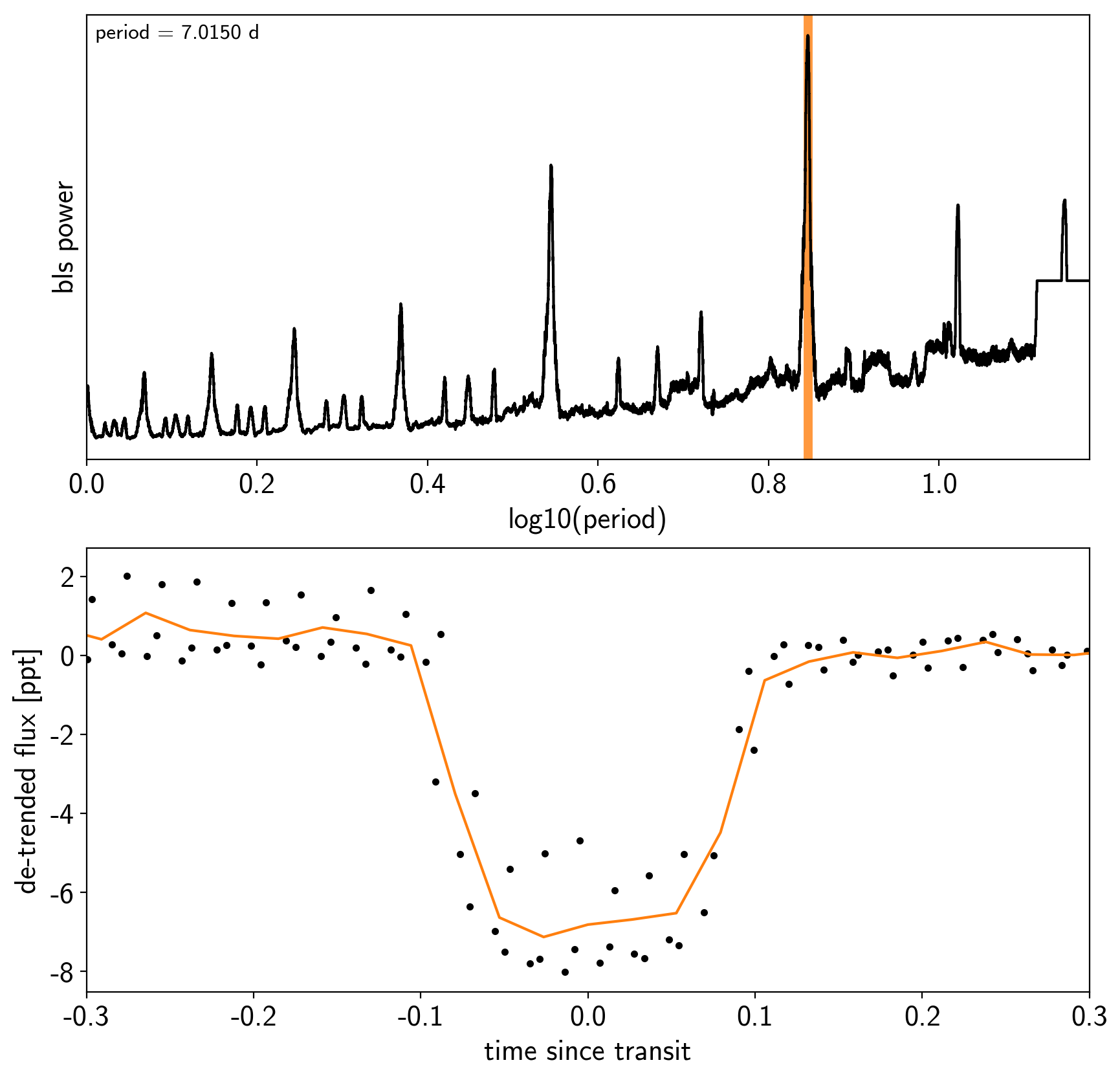
from astropy.stats import BoxLeastSquares

period_grid = np.exp(np.linspace(np.log(1), np.log(15), 50000))

bls = BoxLeastSquares(time, sap_flux - pld_flux)
bls_power = bls.power(period_grid, 0.1, oversample=20)

# Save the highest peak as the planet candidate
index = np.argmax(bls_power.power)
bls_period = bls_power.period[index]
bls_t0 = bls_power.transit_time[index]
bls_depth = bls_power.depth[index]
transit_mask = bls.transit_mask(time, bls_period, 0.2, bls_t0)

fig, axes = plt.subplots(2, 1, figsize=(10, 10))

# Plot the periodogram
ax = axes[0]
ax.axvline(np.log10(bls_period), color="C1", lw=5, alpha=0.8)
ax.plot(np.log10(bls_power.period), bls_power.power, "k")
ax.annotate("period = {0:.4f} d".format(bls_period),
            (0, 1), xycoords="axes fraction",
            xytext=(5, -5), textcoords="offset points",
            va="top", ha="left", fontsize=12)
ax.set_ylabel("bls power")
ax.set_yticks([])
ax.set_xlim(np.log10(period_grid.min()), np.log10(period_grid.max()))
ax.set_xlabel("log10(period)")

# Plot the folded transit
ax = axes[1]
x_fold = (time - bls_t0 + 0.5*bls_period)%bls_period - 0.5*bls_period
m = np.abs(x_fold) < 0.4
ax.plot(x_fold[m], sap_flux[m] - pld_flux[m], ".k")

# Overplot the phase binned light curve
bins = np.linspace(-0.41, 0.41, 32)
denom, _ = np.histogram(x_fold, bins)
num, _ = np.histogram(x_fold, bins, weights=sap_flux - pld_flux)
denom[num == 0] = 1.0
ax.plot(0.5*(bins[1:] + bins[:-1]), num / denom, color="C1")

ax.set_xlim(-0.3, 0.3)
ax.set_ylabel("de-trended flux [ppt]")
ax.set_xlabel("time since transit");
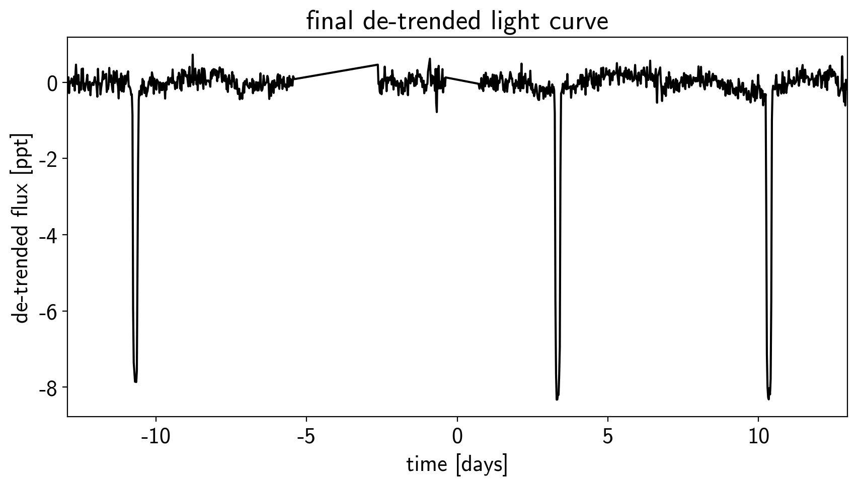
m = ~transit_mask
XTX = np.dot(X_pld[m].T, X_pld[m])
w_pld = np.linalg.solve(XTX, np.dot(X_pld[m].T, sap_flux[m]))
pld_flux = np.dot(X_pld, w_pld)

x = np.ascontiguousarray(time, dtype=np.float64)
y = np.ascontiguousarray(sap_flux-pld_flux, dtype=np.float64)

plt.figure(figsize=(10, 5))
plt.plot(time, y, "k")
plt.xlabel("time [days]")
plt.ylabel("de-trended flux [ppt]")
plt.title("final de-trended light curve")
plt.xlim(time.min(), time.max());
import exoplanet as xo
import pymc3 as pm
import theano.tensor as tt

def build_model(mask=None, start=None):
    if mask is None:
        mask = np.ones(len(x), dtype=bool)
    with pm.Model() as model:

        # Parameters for the stellar properties
        mean = pm.Normal("mean", mu=0.0, sd=10.0)
        u_star = xo.distributions.QuadLimbDark("u_star")

        # Stellar parameters from TIC
        M_star_huang = 1.094, 0.039
        R_star_huang = 1.10, 0.023
        m_star = pm.Normal("m_star", mu=tic_mass[0], sd=tic_mass[1])
        r_star = pm.Normal("r_star", mu=tic_radius[0], sd=tic_radius[1])

        # Prior to require physical parameters
        pm.Potential("m_star_prior", tt.switch(m_star > 0, 0, -np.inf))
        pm.Potential("r_star_prior", tt.switch(r_star > 0, 0, -np.inf))

        # Orbital parameters for the planets
        logP = pm.Normal("logP", mu=np.log(bls_period), sd=1)
        t0 = pm.Normal("t0", mu=bls_t0, sd=1)
        b = pm.Uniform("b", lower=0, upper=1, testval=0.5)
        logr = pm.Normal("logr", sd=1.0,
                         mu=0.5*np.log(1e-3*np.array(bls_depth))+np.log(tic_radius[0]))
        r_pl = pm.Deterministic("r_pl", tt.exp(logr))
        ror = pm.Deterministic("ror", r_pl / r_star)

        # This is the eccentricity prior from Kipping (2013):
        # https://arxiv.org/abs/1306.4982
        ecc = pm.Beta("ecc", alpha=0.867, beta=3.03, testval=0.1)
        omega = xo.distributions.Angle("omega")

        # Transit jitter & GP parameters
        logs2 = pm.Normal("logs2", mu=np.log(np.var(y[mask])), sd=10)
        logw0_guess = np.log(2*np.pi/10)
        logw0 = pm.Normal("logw0", mu=logw0_guess, sd=10)

        # We'll parameterize using the maximum power (S_0 * w_0^4) instead of
        # S_0 directly because this removes some of the degeneracies between
        # S_0 and omega_0
        logpower = pm.Normal("logpower",
                             mu=np.log(np.var(y[mask]))+4*logw0_guess,
                             sd=10)
        logS0 = pm.Deterministic("logS0", logpower - 4 * logw0)

        # Tracking planet parameters
        period = pm.Deterministic("period", tt.exp(logP))

        # Orbit model
        orbit = xo.orbits.KeplerianOrbit(
            r_star=r_star, m_star=m_star,
            period=period, t0=t0, b=b,
            ecc=ecc, omega=omega)
        pm.Deterministic("a", orbit.a_planet)
        pm.Deterministic("incl", orbit.incl)

        # Compute the model light curve using starry
        light_curves = xo.StarryLightCurve(u_star).get_light_curve(
            orbit=orbit, r=r_pl, t=x[mask], texp=texp)*1e3
        light_curve = pm.math.sum(light_curves, axis=-1) + mean
        pm.Deterministic("light_curves", light_curves)

        # GP model for the light curve
        kernel = xo.gp.terms.SHOTerm(log_S0=logS0, log_w0=logw0, Q=1/np.sqrt(2))
        gp = xo.gp.GP(kernel, x[mask], tt.exp(logs2) + tt.zeros(mask.sum()), J=2)
        pm.Potential("transit_obs", gp.log_likelihood(y[mask] - light_curve))
        pm.Deterministic("gp_pred", gp.predict())

        # Fit for the maximum a posteriori parameters, I've found that I can get
        # a better solution by trying different combinations of parameters in turn
        if start is None:
            start = model.test_point
        map_soln = xo.optimize(start=start, vars=[b])
        map_soln = xo.optimize(start=map_soln, vars=[logs2, logpower, logw0])
        map_soln = xo.optimize(start=map_soln, vars=[logr])
        map_soln = xo.optimize(start=map_soln)

    return model, map_soln

model0, map_soln0 = build_model()
optimizing logp for variables: ['b_interval__']
message: Optimization terminated successfully.
logp: -1187.4649971584893 -> -1167.1812080299917
optimizing logp for variables: ['logw0', 'logpower', 'logs2']
message: Optimization terminated successfully.
logp: -1167.181208029992 -> 66.71318590430374
optimizing logp for variables: ['logr']
message: Optimization terminated successfully.
logp: 66.71318590430374 -> 106.91173137171472
optimizing logp for variables: ['logpower', 'logw0', 'logs2', 'omega_angle__', 'ecc_logodds__', 'logr', 'b_interval__', 't0', 'logP', 'r_star', 'm_star', 'u_star_quadlimbdark__', 'mean']
message: Desired error not necessarily achieved due to precision loss.
logp: 106.9117313717145 -> 343.1349315401228
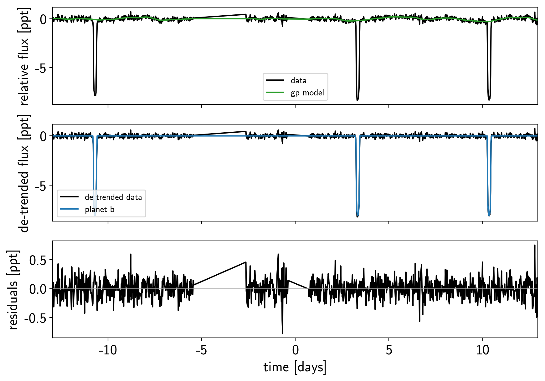
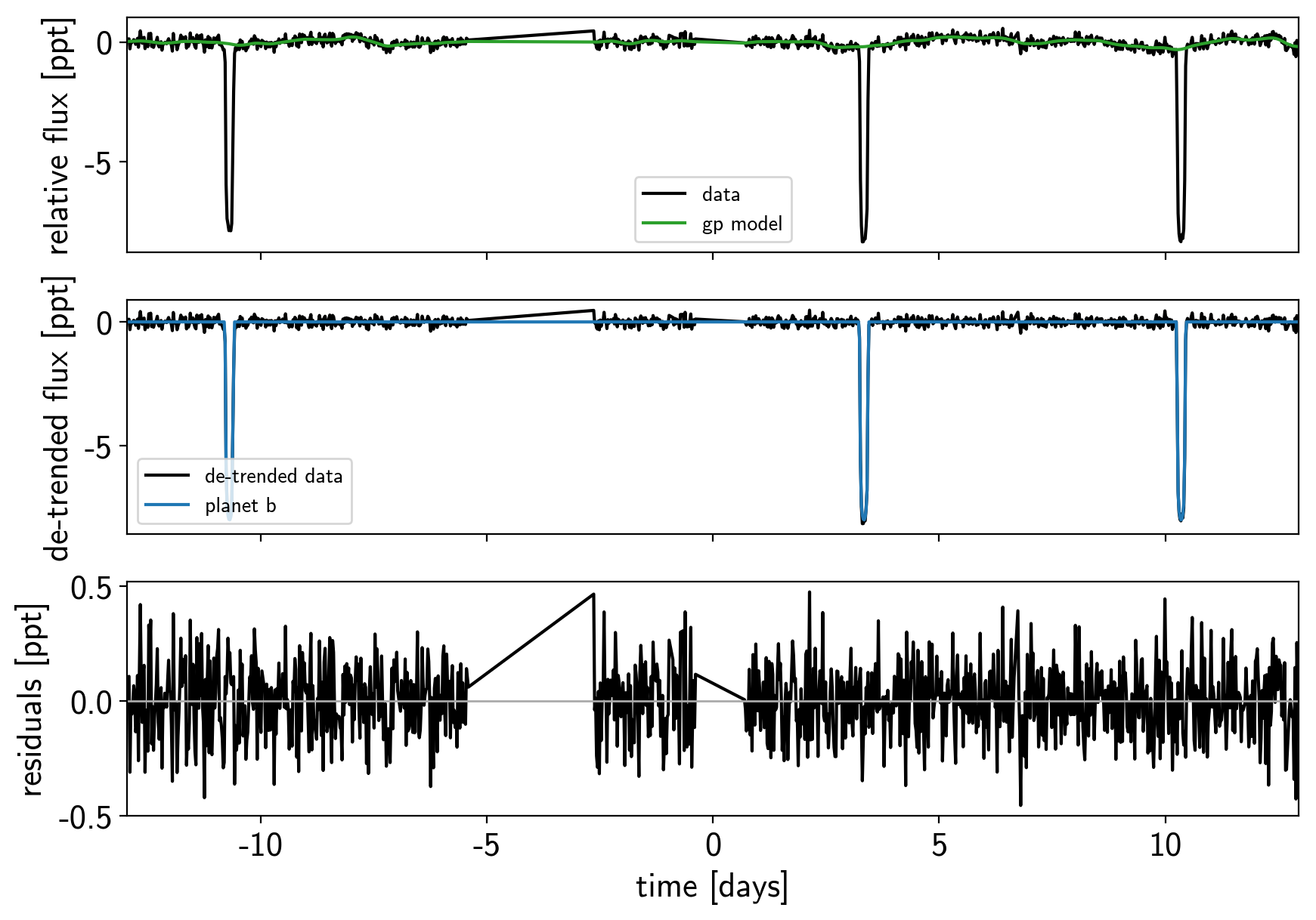
def plot_light_curve(soln, mask=None):
    if mask is None:
        mask = np.ones(len(x), dtype=bool)

    fig, axes = plt.subplots(3, 1, figsize=(10, 7), sharex=True)

    ax = axes[0]
    ax.plot(x[mask], y[mask], "k", label="data")
    gp_mod = soln["gp_pred"] + soln["mean"]
    ax.plot(x[mask], gp_mod, color="C2", label="gp model")
    ax.legend(fontsize=10)
    ax.set_ylabel("relative flux [ppt]")

    ax = axes[1]
    ax.plot(x[mask], y[mask] - gp_mod, "k", label="de-trended data")
    for i, l in enumerate("b"):
        mod = soln["light_curves"][:, i]
        ax.plot(x[mask], mod, label="planet {0}".format(l))
    ax.legend(fontsize=10, loc=3)
    ax.set_ylabel("de-trended flux [ppt]")

    ax = axes[2]
    mod = gp_mod + np.sum(soln["light_curves"], axis=-1)
    ax.plot(x[mask], y[mask] - mod, "k")
    ax.axhline(0, color="#aaaaaa", lw=1)
    ax.set_ylabel("residuals [ppt]")
    ax.set_xlim(x[mask].min(), x[mask].max())
    ax.set_xlabel("time [days]")

    return fig

plot_light_curve(map_soln0);
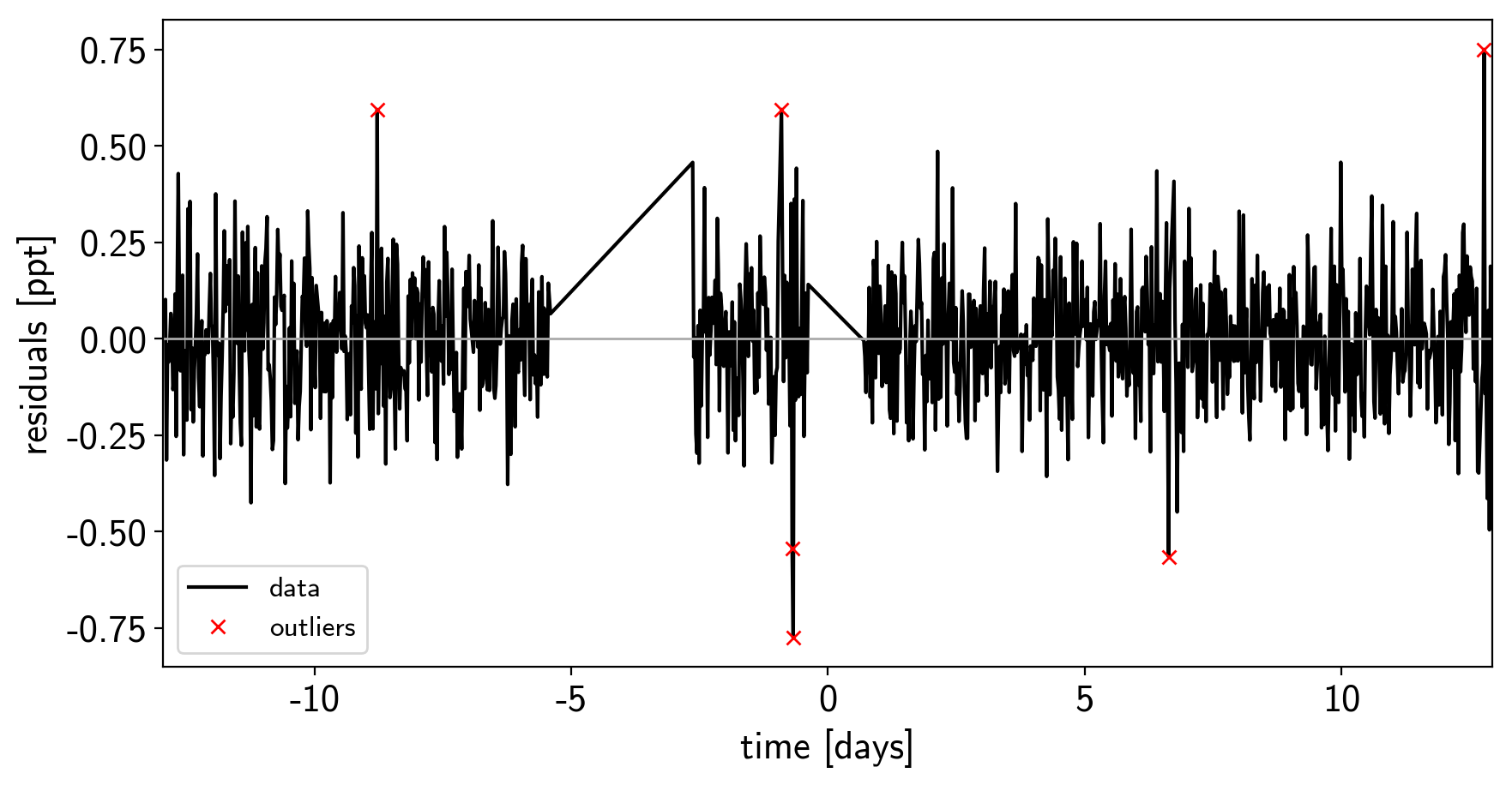
mod = map_soln0["gp_pred"] + map_soln0["mean"] + np.sum(map_soln0["light_curves"], axis=-1)
resid = y - mod
rms = np.sqrt(np.median(resid**2))
mask = np.abs(resid) < 5 * rms

plt.figure(figsize=(10, 5))
plt.plot(x, resid, "k", label="data")
plt.plot(x[~mask], resid[~mask], "xr", label="outliers")
plt.axhline(0, color="#aaaaaa", lw=1)
plt.ylabel("residuals [ppt]")
plt.xlabel("time [days]")
plt.legend(fontsize=12, loc=3)
plt.xlim(x.min(), x.max());
model, map_soln = build_model(mask, map_soln0)
plot_light_curve(map_soln, mask);
optimizing logp for variables: ['b_interval__']
message: Optimization terminated successfully.
logp: 385.5369927156757 -> 385.5369927169309
optimizing logp for variables: ['logw0', 'logpower', 'logs2']
message: Optimization terminated successfully.
logp: 385.53699271693114 -> 388.4181918654495
optimizing logp for variables: ['logr']
message: Optimization terminated successfully.
logp: 388.4181918654495 -> 388.4388036404506
optimizing logp for variables: ['logpower', 'logw0', 'logs2', 'omega_angle__', 'ecc_logodds__', 'logr', 'b_interval__', 't0', 'logP', 'r_star', 'm_star', 'u_star_quadlimbdark__', 'mean']
message: Desired error not necessarily achieved due to precision loss.
logp: 388.4388036404497 -> 388.4492815037509
np.random.seed(12345)
sampler = xo.PyMC3Sampler(window=100, start=300, finish=500)
with model:
    burnin = sampler.tune(tune=3500, start=map_soln,
                          step_kwargs=dict(target_accept=0.9),
                          chains=4)
Sampling 4 chains: 100%|██████████| 1208/1208 [04:10<00:00,  1.77draws/s]
Sampling 4 chains: 100%|██████████| 408/408 [00:38<00:00,  2.10draws/s]
Sampling 4 chains: 100%|██████████| 808/808 [01:20<00:00,  2.08draws/s]
The chain contains only diverging samples. The model is probably misspecified.
Sampling 4 chains: 100%|██████████| 1608/1608 [02:47<00:00,  2.86draws/s]
The chain contains only diverging samples. The model is probably misspecified.
Sampling 4 chains: 100%|██████████| 3208/3208 [06:09<00:00,  2.42draws/s]
Sampling 4 chains: 100%|██████████| 6808/6808 [12:44<00:00,  2.46draws/s]
Sampling 4 chains: 100%|██████████| 2008/2008 [04:04<00:00,  2.72draws/s]
with model:
    trace = sampler.sample(draws=1000, chains=4)
Multiprocess sampling (4 chains in 4 jobs)
NUTS: [logpower, logw0, logs2, omega, ecc, logr, b, t0, logP, r_star, m_star, u_star, mean]
Sampling 4 chains: 100%|██████████| 4000/4000 [06:26<00:00,  5.32draws/s]
There were 75 divergences after tuning. Increase target_accept or reparameterize.
The acceptance probability does not match the target. It is 0.8345794868227246, but should be close to 0.9. Try to increase the number of tuning steps.
There were 93 divergences after tuning. Increase target_accept or reparameterize.
The acceptance probability does not match the target. It is 0.81400390534251, but should be close to 0.9. Try to increase the number of tuning steps.
There were 88 divergences after tuning. Increase target_accept or reparameterize.
There were 137 divergences after tuning. Increase target_accept or reparameterize.
The acceptance probability does not match the target. It is 0.8255575460693226, but should be close to 0.9. Try to increase the number of tuning steps.
The number of effective samples is smaller than 10% for some parameters.
pm.summary(trace, varnames=["logw0", "logS0", "logs2", "omega", "ecc", "r_pl", "b", "t0", "logP", "r_star", "m_star", "u_star", "mean"])
| mean | sd | mc_error | hpd_2.5 | hpd_97.5 | n_eff | Rhat | |
|---|---|---|---|---|---|---|---|
| logw0 | 1.153784 | 0.239958 | 4.483356e-03 | 0.657851 | 1.602863 | 2494.944595 | 1.000564 |
| logS0 | -4.966758 | 0.417187 | 8.941177e-03 | -5.727554 | -4.131493 | 2114.231030 | 1.000331 |
| logs2 | -3.704235 | 0.046502 | 8.866861e-04 | -3.797804 | -3.615236 | 2730.479241 | 1.000054 |
| omega | 0.732818 | 1.703787 | 6.510296e-02 | -2.995388 | 3.051943 | 569.555903 | 0.999763 |
| ecc | 0.201140 | 0.148681 | 6.683953e-03 | 0.000017 | 0.486072 | 316.482457 | 1.003757 |
| r_pl | 0.150164 | 0.017211 | 5.095313e-04 | 0.117328 | 0.185128 | 950.454432 | 1.000284 |
| b | 0.482573 | 0.173359 | 6.206205e-03 | 0.122164 | 0.725565 | 734.499407 | 1.000846 |
| t0 | -3.673688 | 0.000808 | 3.513089e-05 | -3.675519 | -3.672016 | 545.856527 | 1.000821 |
| logP | 1.947507 | 0.000030 | 6.791008e-07 | 1.947450 | 1.947567 | 2016.102978 | 0.999553 |
| r_star | 1.769657 | 0.188341 | 5.629718e-03 | 1.408608 | 2.151118 | 924.304048 | 1.000228 |
| m_star | 1.369237 | 0.239829 | 5.796899e-03 | 0.919993 | 1.834767 | 2433.985473 | 1.001036 |
| u_star__0 | 0.158632 | 0.123987 | 2.803874e-03 | 0.000732 | 0.420283 | 1786.454918 | 0.999961 |
| u_star__1 | 0.471364 | 0.278805 | 7.783860e-03 | -0.084607 | 0.940409 | 1160.740321 | 1.000235 |
| mean | -0.010038 | 0.026501 | 5.858189e-04 | -0.061976 | 0.042051 | 1948.173185 | 1.000639 |
# Compute the GP prediction
gp_mod = np.median(trace["gp_pred"] + trace["mean"][:, None], axis=0)
# Get the posterior median orbital parameters
p = np.median(trace["period"])
t0 = np.median(trace["t0"])
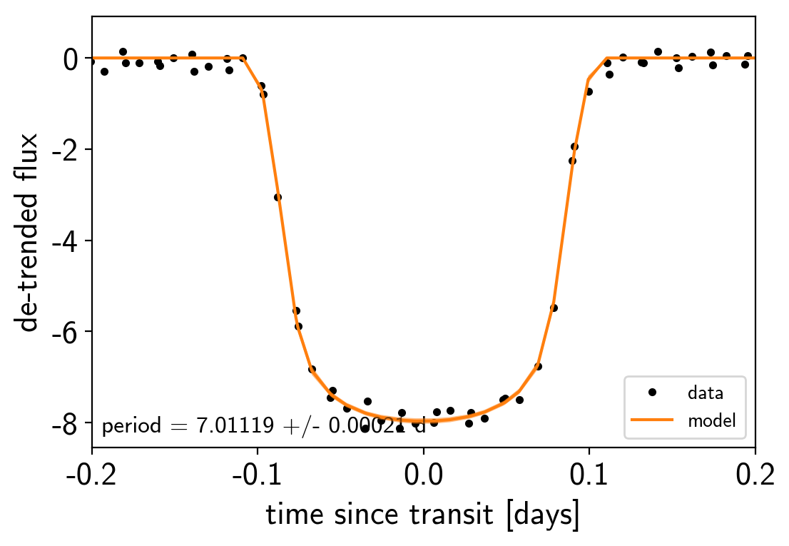
# Plot the folded data
x_fold = (x[mask] - t0 + 0.5*p) % p - 0.5*p
plt.plot(x_fold, y[mask] - gp_mod, ".k", label="data", zorder=-1000)
# Plot the folded model
inds = np.argsort(x_fold)
inds = inds[np.abs(x_fold)[inds] < 0.3]
pred = trace["light_curves"][:, inds, 0]
pred = np.percentile(pred, [16, 50, 84], axis=0)
plt.plot(x_fold[inds], pred[1], color="C1", label="model")
art = plt.fill_between(x_fold[inds], pred[0], pred[2], color="C1", alpha=0.5,
zorder=1000)
art.set_edgecolor("none")
# Annotate the plot with the planet's period
txt = "period = {0:.5f} +/- {1:.5f} d".format(
np.mean(trace["period"]), np.std(trace["period"]))
plt.annotate(txt, (0, 0), xycoords="axes fraction",
xytext=(5, 5), textcoords="offset points",
ha="left", va="bottom", fontsize=12)
plt.legend(fontsize=10, loc=4)
plt.xlim(-0.5*p, 0.5*p)
plt.xlabel("time since transit [days]")
plt.ylabel("de-trended flux")
plt.xlim(-0.2, 0.2);
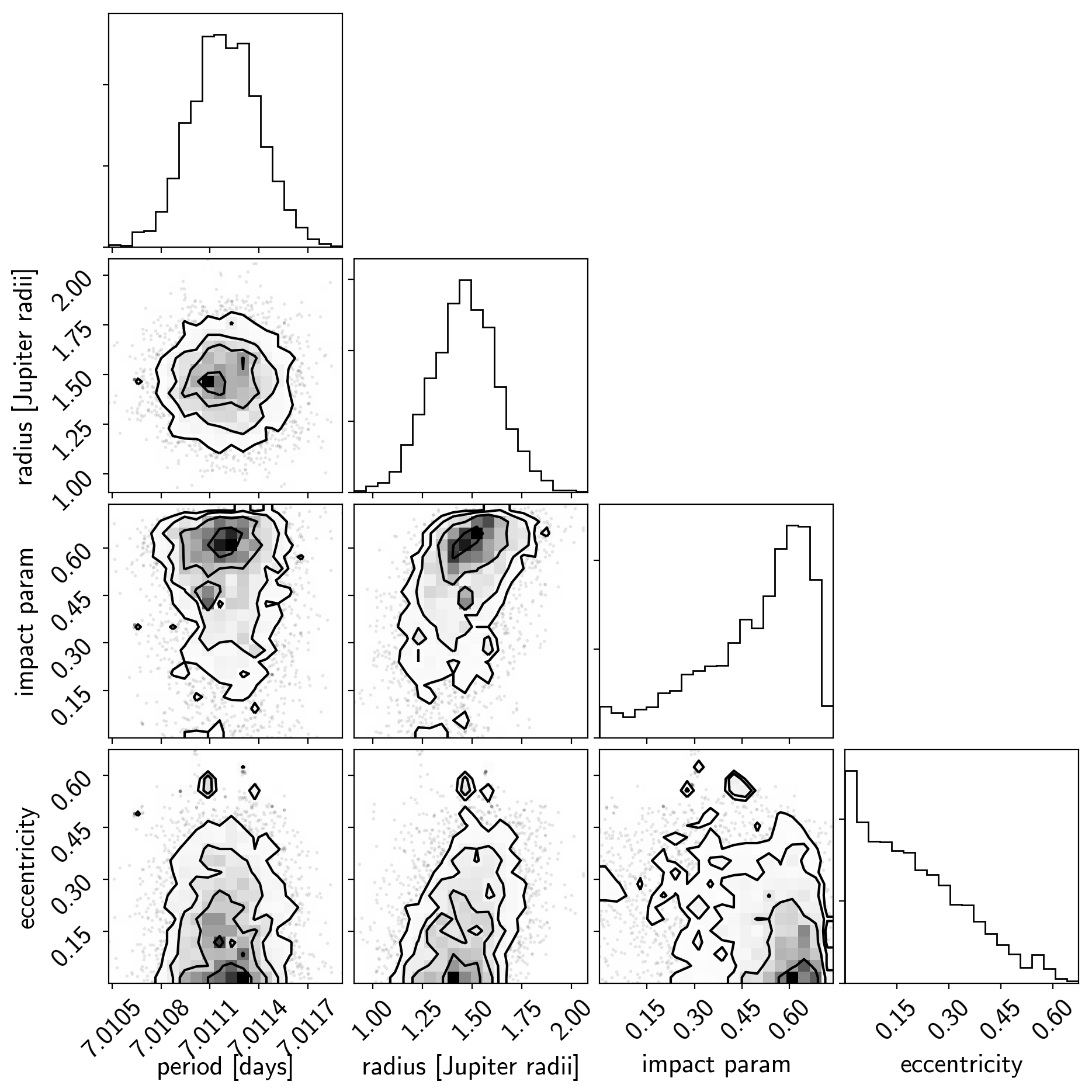
import corner
import astropy.units as u
varnames = ["period", "b", "ecc", "r_pl"]
samples = pm.trace_to_dataframe(trace, varnames=varnames)

# Convert the radius to Earth radii
samples["r_pl"] = (np.array(samples["r_pl"]) * u.R_sun).to(u.R_jupiter).value

corner.corner(
    samples[["period", "r_pl", "b", "ecc"]],
    labels=["period [days]", "radius [Jupiter radii]", "impact param", "eccentricity"]);
aor = -trace["a"] / trace["r_star"]
e = trace["ecc"]
w = trace["omega"]
i = trace["incl"]
b = trace["b"]
k = trace["r_pl"] / trace["r_star"]
P = trace["period"]
T_tot = P/np.pi * np.arcsin(np.sqrt(1 - b**2) / np.sin(i) / aor)
dur = T_tot * np.sqrt(1 - e**2) / (1 + e * np.sin(w))
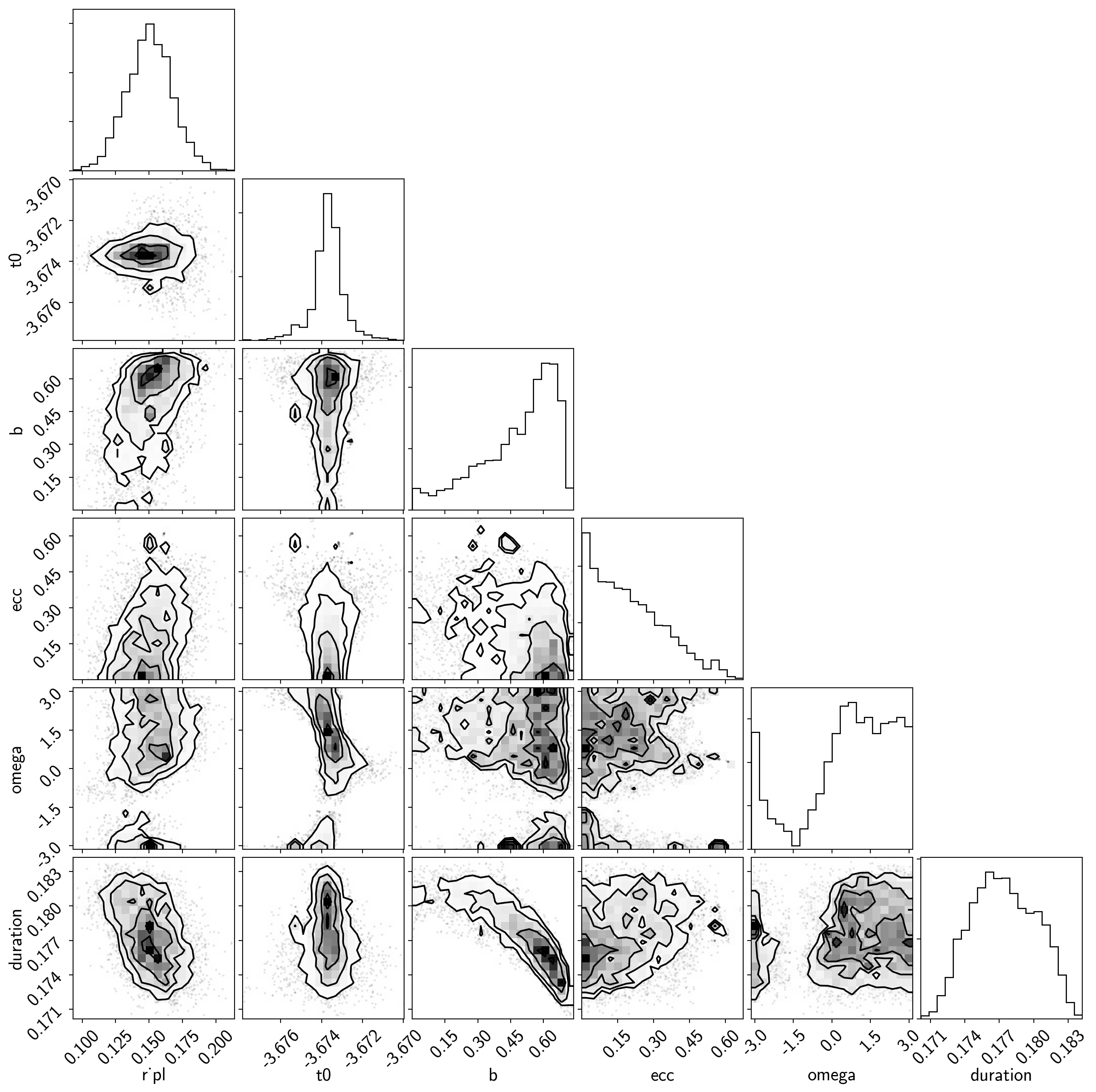
samples = pm.trace_to_dataframe(trace, varnames=["r_pl", "t0", "b", "ecc", "omega"])
samples["duration"] = dur
corner.corner(samples);