Note
This tutorial was generated from an IPython notebook that can be downloaded here.
Scalable Gaussian processes in PyMC3
theano version: 1.0.4
pymc3 version: 3.6
exoplanet version: 0.1.6
PyMC3 has support for Gaussian Processes (GPs), but this implementation is too slow for many applications in time series astrophysics. So exoplanet comes with an implementation of scalable GPs powered by celerite. More information about the algorithm can be found in the celerite docs and in the papers (Paper 1 and Paper 2), but this tutorial will give a hands on demo of how to use celerite in PyMC3.
Note
For the best results, we generally recommend the use of the exoplanet.gp.terms.SHOTerm, exoplanet.gp.terms.Matern32Term, and exoplanet.gp.terms.RotationTerm “terms” because the other terms tend to have unphysical behavior at high frequency.
Let’s start with the quickstart demo from the celerite
docs.
We’ll fit the following simulated dataset using the sum of two
exoplanet.gp.terms.SHOTerm objects.
First, generate the simulated data:
import numpy as np
import matplotlib.pyplot as plt
np.random.seed(42)

t = np.sort(np.append(
    np.random.uniform(0, 3.8, 57),
    np.random.uniform(5.5, 10, 68),
))  # The input coordinates must be sorted
yerr = np.random.uniform(0.08, 0.22, len(t))
y = 0.2 * (t-5) + np.sin(3*t + 0.1*(t-5)**2) + yerr * np.random.randn(len(t))

true_t = np.linspace(0, 10, 5000)
true_y = 0.2 * (true_t-5) + np.sin(3*true_t + 0.1*(true_t-5)**2)

plt.errorbar(t, y, yerr=yerr, fmt=".k", capsize=0, label="data")
plt.plot(true_t, true_y, "k", lw=1.5, alpha=0.3, label="truth")
plt.legend(fontsize=12)
plt.xlabel("t")
plt.ylabel("y")
plt.xlim(0, 10)
plt.ylim(-2.5, 2.5);
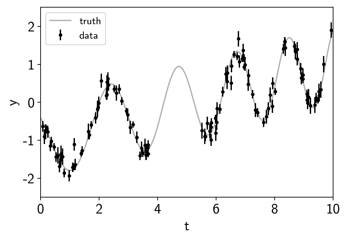
This plot shows the simulated data as black points with error bars and the true function is shown as a gray line.
Now let’s build the PyMC3 model that we’ll use to fit the data. We can see that there’s some roughly periodic signal in the data as well as a longer term trend. To capture these two features, we will model this as a mixture of two stochastically driven simple harmonic oscillators (SHO) with the power spectrum:
The first term is exoplanet.gp.terms.SHOterm with
\(Q=1/\sqrt{2}\) and the second is regular
exoplanet.gp.terms.SHOterm. This model has 5 free parameters
(\(S_1\), \(\omega_1\), \(S_2\), \(\omega_2\), and
\(Q\)) and they must all be positive so we’ll fit for the log of
each parameter. Using exoplanet, this is how you would build this
model, choosing more or less arbitrary initial values for the
parameters.
import pymc3 as pm
import theano.tensor as tt
from exoplanet.gp import terms, GP

with pm.Model() as model:

    logS1 = pm.Normal("logS1", mu=0.0, sd=15.0, testval=np.log(np.var(y)))
    logw1 = pm.Normal("logw1", mu=0.0, sd=15.0, testval=np.log(3.0))
    logS2 = pm.Normal("logS2", mu=0.0, sd=15.0, testval=np.log(np.var(y)))
    logw2 = pm.Normal("logw2", mu=0.0, sd=15.0, testval=np.log(3.0))
    logQ = pm.Normal("logQ", mu=0.0, sd=15.0, testval=0)

    # Set up the kernel an GP
    kernel = terms.SHOTerm(log_S0=logS1, log_w0=logw1, Q=1.0/np.sqrt(2))
    kernel += terms.SHOTerm(log_S0=logS2, log_w0=logw2, log_Q=logQ)
    gp = GP(kernel, t, yerr**2)

    # Add a custom "potential" (log probability function) with the GP likelihood
    pm.Potential("gp", gp.log_likelihood(y))
A few comments here:
- The
terminterface in exoplanet only accepts keyword arguments with names given by theparameter_namesproperty of the term. But it will also interpret keyword arguments with the name prefaced bylog_to be the log of the parameter. For example, in this case, we usedlog_S0as the parameter for each term, butS0=tt.exp(log_S0)would have been equivalent. This is useful because many of the parameters are required to be positive so fitting the log of those parameters is often best. - The third argument to the
exoplanet.gp.GPconstructor should be the variance to add along the diagonal, not the standard deviation as in the original celerite implementation. - Finally, the
exoplanet.gp.GPconstructor takes an optional argumentJwhich specifies the width of the problem if it is known at compile time. Just to be confusing, this is actually two times theJfrom the celerite paper. There are various technical reasons why this is difficult to work out in general and this code will always work if you don’t provide a value forJ, but you can get much better performance (especially for smallJ) if you know what it will be for your problem. In general, most terms costJ=2with the exception of aexoplanet.gp.terms.RealTerm(which costs J=1) and aexoplanet.gp.terms.RotationTerm(which costs J=4).
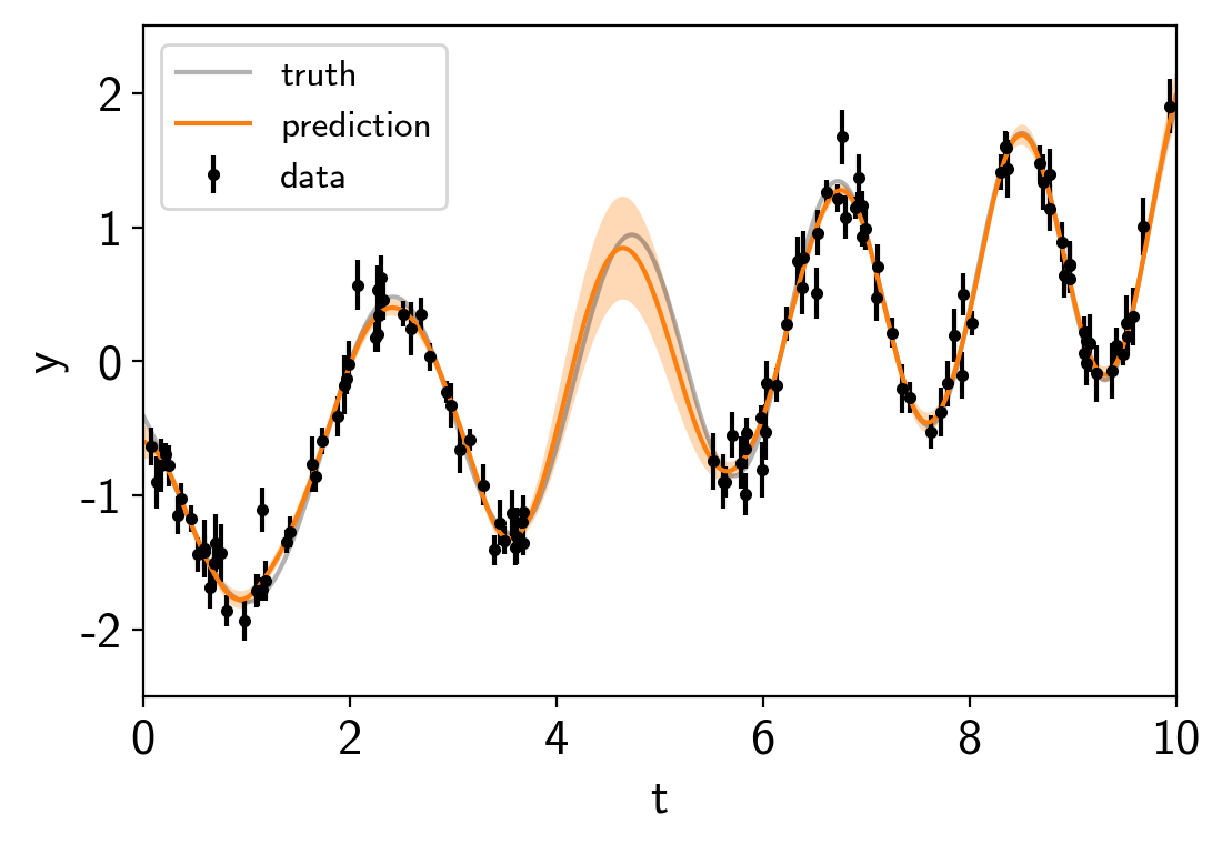
To start, let’s fit for the maximum a posteriori (MAP) parameters and look the the predictions that those make.
import exoplanet as xo
with model:
    map_soln = xo.optimize(start=model.test_point)
optimizing logp for variables: ['logQ', 'logw2', 'logS2', 'logw1', 'logS1']
message: Optimization terminated successfully.
logp: -41.068631281249985 -> -1.6509594267148024
We’ll use the exoplanet.eval_in_model() function to evaluate the
MAP GP model.
with model:
    mu, var = xo.eval_in_model(gp.predict(true_t, return_var=True), map_soln)
plt.errorbar(t, y, yerr=yerr, fmt=".k", capsize=0, label="data")
plt.plot(true_t, true_y, "k", lw=1.5, alpha=0.3, label="truth")

# Plot the prediction and the 1-sigma uncertainty
sd = np.sqrt(var)
art = plt.fill_between(true_t, mu+sd, mu-sd, color="C1", alpha=0.3)
art.set_edgecolor("none")
plt.plot(true_t, mu, color="C1", label="prediction")

plt.legend(fontsize=12)
plt.xlabel("t")
plt.ylabel("y")
plt.xlim(0, 10)
plt.ylim(-2.5, 2.5);
Now we can sample this model using PyMC3. There are strong covariances
between the parameters so we’ll use the custom
exoplanet.PyMC3Sampler to fit for these covariances during
burn-in.
from exoplanet.sampling import PyMC3Sampler

sampler = PyMC3Sampler()

with model:
    burnin = sampler.tune(tune=1000, chains=2, start=map_soln)
    trace = sampler.sample(draws=2000, chains=2)
Sampling 2 chains: 100%|██████████| 154/154 [00:03<00:00, 47.19draws/s]
Sampling 2 chains: 100%|██████████| 54/54 [00:00<00:00, 85.64draws/s]
Sampling 2 chains: 100%|██████████| 104/104 [00:00<00:00, 269.18draws/s]
Sampling 2 chains: 100%|██████████| 204/204 [00:00<00:00, 349.71draws/s]
Sampling 2 chains: 100%|██████████| 404/404 [00:01<00:00, 386.57draws/s]
Sampling 2 chains: 100%|██████████| 1104/1104 [00:02<00:00, 382.38draws/s]
Sampling 2 chains: 100%|██████████| 104/104 [00:00<00:00, 279.67draws/s]
Multiprocess sampling (2 chains in 4 jobs)
NUTS: [logQ, logw2, logS2, logw1, logS1]
Sampling 2 chains: 100%|██████████| 4000/4000 [00:07<00:00, 550.60draws/s]
There were 25 divergences after tuning. Increase target_accept or reparameterize.
There were 28 divergences after tuning. Increase target_accept or reparameterize.
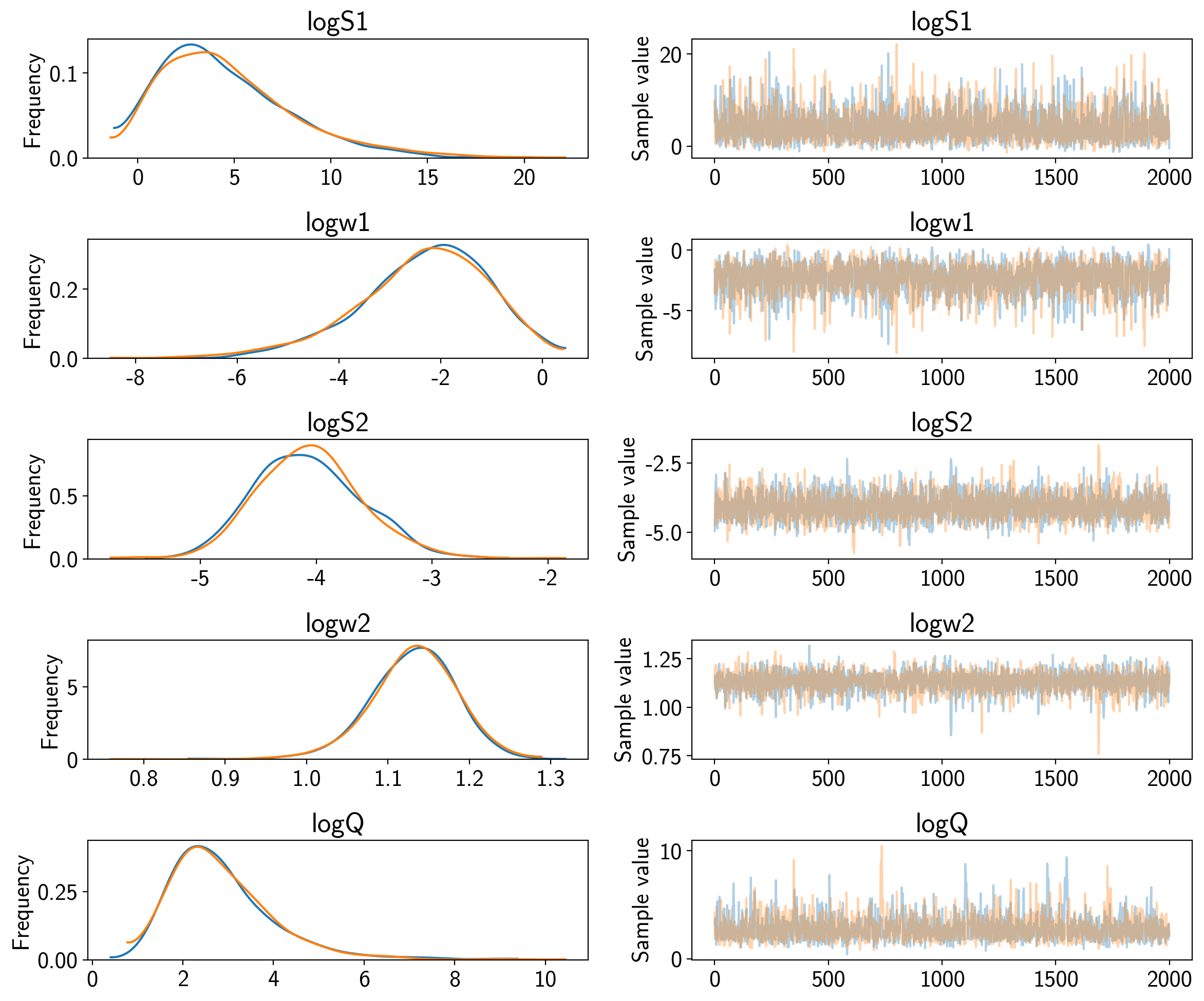
Now we can compute the standard PyMC3 convergence statistics (using
pymc3.summary) and make a trace plot (using pymc3.traceplot).
pm.traceplot(trace)
pm.summary(trace)
| mean | sd | mc_error | hpd_2.5 | hpd_97.5 | n_eff | Rhat | |
|---|---|---|---|---|---|---|---|
| logS1 | 4.617327 | 3.461732 | 0.074461 | -0.669599 | 11.641176 | 1796.383040 | 1.001029 |
| logw1 | -2.357079 | 1.278509 | 0.028268 | -4.906263 | -0.031826 | 1732.776588 | 1.000904 |
| logS2 | -4.065707 | 0.460787 | 0.009704 | -4.894512 | -3.126594 | 1964.834714 | 0.999994 |
| logw2 | 1.130031 | 0.051583 | 0.001032 | 1.026167 | 1.226491 | 2190.463087 | 0.999914 |
| logQ | 2.848372 | 1.140540 | 0.034108 | 1.029216 | 5.016399 | 1023.945161 | 0.999776 |
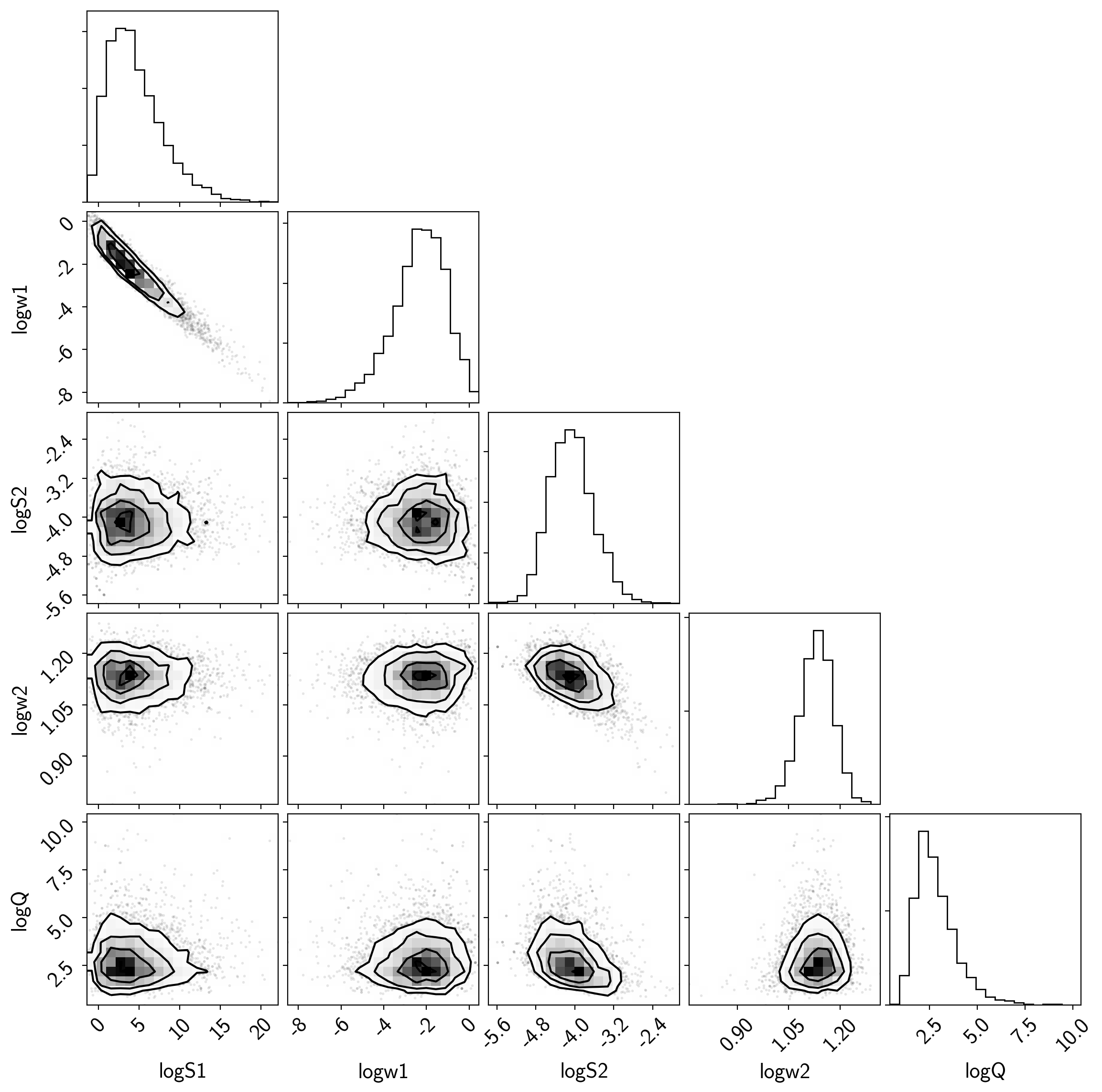
That all looks pretty good, but I like to make two other results plots: (1) a corner plot and (2) a posterior predictive plot.
The corner plot is easy using pymc3.trace_to_dataframe and I find it
useful for understanding the covariances between parameters when
debugging.
import corner
samples = pm.trace_to_dataframe(trace)
corner.corner(samples);
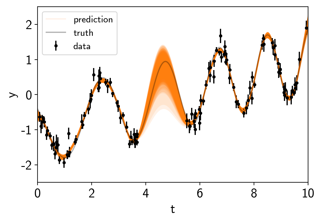
The “posterior predictive” plot that I like to make isn’t the same as a
“posterior predictive check” (which can be a good thing to do too).
Instead, I like to look at the predictions of the model in the space of
the data. We could have saved these predictions using a
pymc3.Deterministic distribution, but that adds some overhead to
each evaluation of the model so instead, we can use
exoplanet.utils.get_samples_from_trace() to loop over a few
random samples from the chain and then the
exoplanet.eval_in_model() function to evaluate the prediction
just for those samples.
# Generate 50 realizations of the prediction sampling randomly from the chain
N_pred = 50
pred_mu = np.empty((N_pred, len(true_t)))
pred_var = np.empty((N_pred, len(true_t)))
with model:
    pred = gp.predict(true_t, return_var=True)
    for i, sample in enumerate(xo.get_samples_from_trace(trace, size=N_pred)):
        pred_mu[i], pred_var[i] = xo.eval_in_model(pred, sample)

# Plot the predictions
for i in range(len(pred_mu)):
    mu = pred_mu[i]
    sd = np.sqrt(pred_var[i])
    label = None if i else "prediction"
    art = plt.fill_between(true_t, mu+sd, mu-sd, color="C1", alpha=0.1)
    art.set_edgecolor("none")
    plt.plot(true_t, mu, color="C1", label=label, alpha=0.1)

plt.errorbar(t, y, yerr=yerr, fmt=".k", capsize=0, label="data")
plt.plot(true_t, true_y, "k", lw=1.5, alpha=0.3, label="truth")
plt.legend(fontsize=12)
plt.xlabel("t")
plt.ylabel("y")
plt.xlim(0, 10)
plt.ylim(-2.5, 2.5);
Citations
As described in the Citing exoplanet & its dependencies tutorial, we can use
exoplanet.citations.get_citations_for_model() to construct an
acknowledgement and BibTeX listing that includes the relevant citations
for this model.
with model:
    txt, bib = xo.citations.get_citations_for_model()
print(txt)
This research made use of textsf{exoplanet} citep{exoplanet} and its
dependencies citep{exoplanet:exoplanet, exoplanet:foremanmackey17,
exoplanet:foremanmackey18, exoplanet:pymc3, exoplanet:theano}.
print("\n".join(bib.splitlines()[:10]) + "\n...")
@misc{exoplanet:exoplanet,
  author = {Dan Foreman-Mackey and
            Geert Barentsen and
            Tom Barclay},
   title = {dfm/exoplanet: exoplanet v0.1.5},
   month = mar,
    year = 2019,
     doi = {10.5281/zenodo.2587222},
     url = {https://doi.org/10.5281/zenodo.2587222}
...