Note
This tutorial was generated from an IPython notebook that can be downloaded here.
theano version: 1.0.4
pymc3 version: 3.7
exoplanet version: 0.2.1
In this tutorial, we will combine many of the previous tutorials to perform a fit of the K2-24 system using the K2 transit data and the RVs from Petigura et al. (2016). This is the same system that we fit in the Radial velocity fitting tutorial and we’ll combine that model with the transit model from the Transit fitting tutorial and the Gaussian Process noise model from the Gaussian process models for stellar variability tutorial.
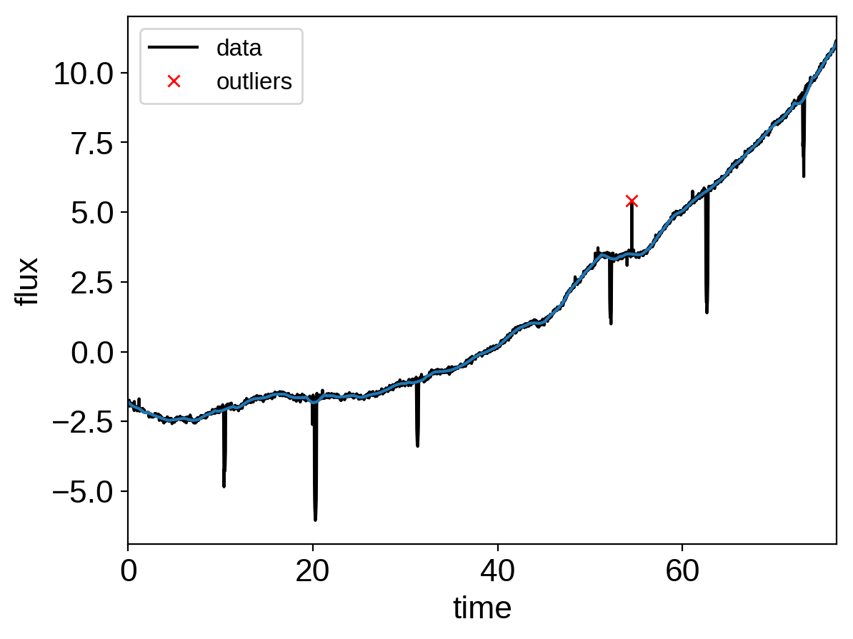
To get started, let’s download the relevant datasets. First, the transit light curve from Everest:
import numpy as np
import matplotlib.pyplot as plt

from astropy.io import fits
from scipy.signal import savgol_filter

# Download the data
lc_url = "https://archive.stsci.edu/hlsps/everest/v2/c02/203700000/71098/hlsp_everest_k2_llc_203771098-c02_kepler_v2.0_lc.fits"
with fits.open(lc_url) as hdus:
    lc = hdus[1].data
    lc_hdr = hdus[1].header

# Work out the exposure time
texp = lc_hdr["FRAMETIM"] * lc_hdr["NUM_FRM"]
texp /= 60.0 * 60.0 * 24.0

# Mask bad data
m = (np.arange(len(lc)) > 100) & np.isfinite(lc["FLUX"]) & np.isfinite(lc["TIME"])
bad_bits=[1, 2, 3, 4, 5, 6, 7, 8, 9, 11, 12, 13, 14, 16, 17]
qual = lc["QUALITY"]
for b in bad_bits:
    m &= qual & 2 ** (b - 1) == 0

# Convert to parts per thousand
x = lc["TIME"][m]
y = lc["FLUX"][m]
mu = np.median(y)
y = (y / mu - 1) * 1e3

# Identify outliers
m = np.ones(len(y), dtype=bool)
for i in range(10):
    y_prime = np.interp(x, x[m], y[m])
    smooth = savgol_filter(y_prime, 101, polyorder=3)
    resid = y - smooth
    sigma = np.sqrt(np.mean(resid**2))
    m0 = np.abs(resid) < 3*sigma
    if m.sum() == m0.sum():
        m = m0
        break
    m = m0

# Only discard positive outliers
m = resid < 3*sigma

# Shift the data so that the K2 data start at t=0. This tends to make the fit
# better behaved since t0 covaries with period.
x_ref = np.min(x[m])
x -= x_ref

# Plot the data
plt.plot(x, y, "k", label="data")
plt.plot(x, smooth)
plt.plot(x[~m], y[~m], "xr", label="outliers")
plt.legend(fontsize=12)
plt.xlim(x.min(), x.max())
plt.xlabel("time")
plt.ylabel("flux")

# Make sure that the data type is consistent
x = np.ascontiguousarray(x[m], dtype=np.float64)
y = np.ascontiguousarray(y[m], dtype=np.float64)
smooth = np.ascontiguousarray(smooth[m], dtype=np.float64)
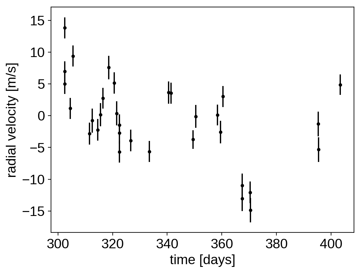
Then the RVs from RadVel:
import pandas as pd

url = "https://raw.githubusercontent.com/California-Planet-Search/radvel/master/example_data/epic203771098.csv"
data = pd.read_csv(url, index_col=0)

# Don't forget to remove the time offset from above!
x_rv = np.array(data.t) - x_ref
y_rv = np.array(data.vel)
yerr_rv = np.array(data.errvel)

plt.errorbar(x_rv, y_rv, yerr=yerr_rv, fmt=".k")
plt.xlabel("time [days]")
plt.ylabel("radial velocity [m/s]");
We can initialize the transit parameters using the box least squares periodogram from AstroPy. (Note: you’ll need AstroPy v3.1 or more recent to use this feature.) A full discussion of transit detection and vetting is beyond the scope of this tutorial so let’s assume that we know that there are two periodic transiting planets in this dataset.
from astropy.timeseries import BoxLeastSquares

m = np.zeros(len(x), dtype=bool)
period_grid = np.exp(np.linspace(np.log(5), np.log(50), 50000))
bls_results = []
periods = []
t0s = []
depths = []

# Compute the periodogram for each planet by iteratively masking out
# transits from the higher signal to noise planets. Here we're assuming
# that we know that there are exactly two planets.
for i in range(2):
    bls = BoxLeastSquares(x[~m], y[~m] - smooth[~m])
    bls_power = bls.power(period_grid, 0.1, oversample=20)
    bls_results.append(bls_power)

    # Save the highest peak as the planet candidate
    index = np.argmax(bls_power.power)
    periods.append(bls_power.period[index])
    t0s.append(bls_power.transit_time[index])
    depths.append(bls_power.depth[index])

    # Mask the data points that are in transit for this candidate
    m |= bls.transit_mask(x, periods[-1], 0.5, t0s[-1])
Let’s plot the initial transit estimates based on these periodograms:
fig, axes = plt.subplots(len(bls_results), 2, figsize=(15, 10))

for i in range(len(bls_results)):
    # Plot the periodogram
    ax = axes[i, 0]
    ax.axvline(np.log10(periods[i]), color="C1", lw=5, alpha=0.8)
    ax.plot(np.log10(bls_results[i].period), bls_results[i].power, "k")
    ax.annotate("period = {0:.4f} d".format(periods[i]),
                (0, 1), xycoords="axes fraction",
                xytext=(5, -5), textcoords="offset points",
                va="top", ha="left", fontsize=12)
    ax.set_ylabel("bls power")
    ax.set_yticks([])
    ax.set_xlim(np.log10(period_grid.min()), np.log10(period_grid.max()))
    if i < len(bls_results) - 1:
        ax.set_xticklabels([])
    else:
        ax.set_xlabel("log10(period)")

    # Plot the folded transit
    ax = axes[i, 1]
    p = periods[i]
    x_fold = (x - t0s[i] + 0.5*p) % p - 0.5*p
    m = np.abs(x_fold) < 0.4
    ax.plot(x_fold[m], y[m] - smooth[m], ".k")

    # Overplot the phase binned light curve
    bins = np.linspace(-0.41, 0.41, 32)
    denom, _ = np.histogram(x_fold, bins)
    num, _ = np.histogram(x_fold, bins, weights=y - smooth)
    denom[num == 0] = 1.0
    ax.plot(0.5*(bins[1:] + bins[:-1]), num / denom, color="C1")

    ax.set_xlim(-0.4, 0.4)
    ax.set_ylabel("relative flux [ppt]")
    if i < len(bls_results) - 1:
        ax.set_xticklabels([])
    else:
        ax.set_xlabel("time since transit")

fig.subplots_adjust(hspace=0.02)
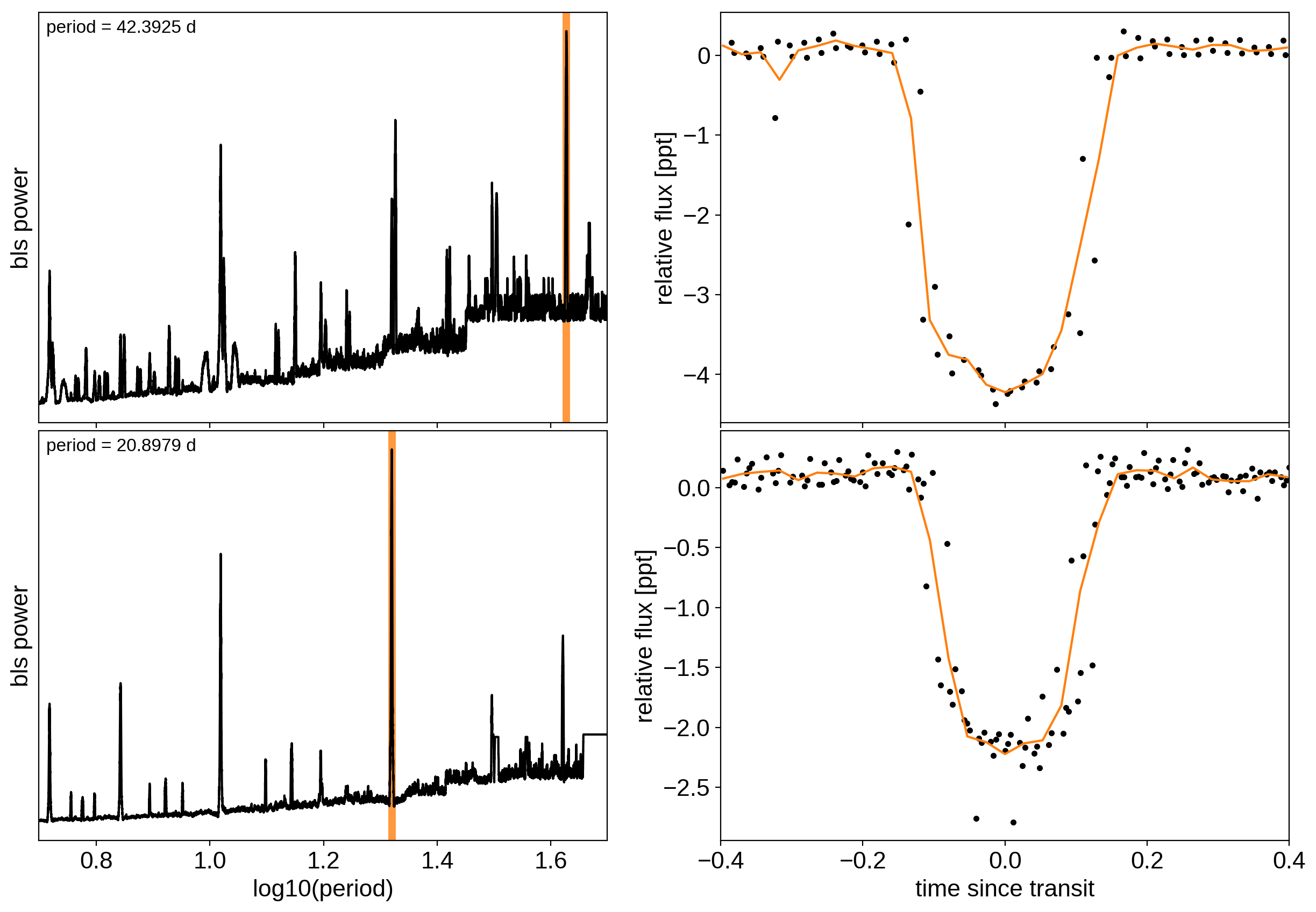
The discovery paper for K2-24 (Petigura et al. (2016)) includes the following estimates of the stellar mass and radius in Solar units:
M_star_petigura = 1.12, 0.05
R_star_petigura = 1.21, 0.11
Finally, using this stellar mass, we can also estimate the minimum masses of the planets given these transit parameters.
import exoplanet as xo
import astropy.units as u

msini = xo.estimate_minimum_mass(periods, x_rv, y_rv, yerr_rv, t0s=t0s, m_star=M_star_petigura[0])
msini = msini.to(u.M_earth)
print(msini)
[32.80060146 23.89885976] earthMass
Now, let’s define our full model in PyMC3. There’s a lot going on here, but I’ve tried to comment it and most of it should be familiar from the previous tutorials (Radial velocity fitting, Transit fitting, Scalable Gaussian processes in PyMC3, and Gaussian process models for stellar variability). In this case, I’ve put the model inside a model “factory” function because we’ll do some sigma clipping below.
import pymc3 as pm
import theano.tensor as tt

t_rv = np.linspace(x_rv.min()-5, x_rv.max()+5, 1000)

def build_model(mask=None, start=None):
    if mask is None:
        mask = np.ones(len(x), dtype=bool)
    with pm.Model() as model:

        # Parameters for the stellar properties
        mean = pm.Normal("mean", mu=0.0, sd=10.0)
        u_star = xo.distributions.QuadLimbDark("u_star")
        BoundedNormal = pm.Bound(pm.Normal, lower=0, upper=3)
        m_star = BoundedNormal("m_star", mu=M_star_petigura[0], sd=M_star_petigura[1])
        r_star = BoundedNormal("r_star", mu=R_star_petigura[0], sd=R_star_petigura[1])

        # Orbital parameters for the planets
        logm = pm.Normal("logm", mu=np.log(msini.value), sd=1, shape=2)
        logP = pm.Normal("logP", mu=np.log(periods), sd=1, shape=2)
        t0 = pm.Normal("t0", mu=np.array(t0s), sd=1, shape=2)
        logr = pm.Normal("logr", mu=0.5*np.log(1e-3*np.array(depths)) + np.log(R_star_petigura[0]),
                         sd=1.0, shape=2)
        r_pl = pm.Deterministic("r_pl", tt.exp(logr))
        ror = pm.Deterministic("ror", r_pl / r_star)
        b = xo.distributions.ImpactParameter("b", ror=ror, shape=2)

        ecc = xo.distributions.eccentricity.vaneylen19(
            "ecc", multi=True, shape=2, testval=np.array([0.01, 0.01]))
        omega = xo.distributions.Angle("omega", shape=2)

        # RV jitter & a quadratic RV trend
        logs_rv = pm.Normal("logs_rv", mu=np.log(np.median(yerr_rv)), sd=5)
        trend = pm.Normal("trend", mu=0, sd=10.0**-np.arange(3)[::-1], shape=3)

        # Transit jitter & GP parameters
        logs2 = pm.Normal("logs2", mu=np.log(np.var(y[mask])), sd=10)
        logw0 = pm.Normal("logw0", mu=0.0, sd=10)
        logSw4 = pm.Normal("logSw4", mu=np.log(np.var(y[mask])), sd=10)

        # Tracking planet parameters
        period = pm.Deterministic("period", tt.exp(logP))
        m_pl = pm.Deterministic("m_pl", tt.exp(logm))

        # Orbit model
        orbit = xo.orbits.KeplerianOrbit(
            r_star=r_star, m_star=m_star,
            period=period, t0=t0, b=b,
            m_planet=xo.units.with_unit(m_pl, msini.unit),
            ecc=ecc, omega=omega)

        # Compute the model light curve using starry
        light_curves = xo.LimbDarkLightCurve(u_star).get_light_curve(
            orbit=orbit, r=r_pl, t=x[mask], texp=texp)*1e3
        light_curve = pm.math.sum(light_curves, axis=-1) + mean
        pm.Deterministic("light_curves", light_curves)

        # GP model for the light curve
        kernel = xo.gp.terms.SHOTerm(log_Sw4=logSw4, log_w0=logw0, Q=1/np.sqrt(2))
        gp = xo.gp.GP(kernel, x[mask], tt.exp(logs2) + tt.zeros(mask.sum()))
        pm.Potential("transit_obs", gp.log_likelihood(y[mask] - light_curve))
        pm.Deterministic("gp_pred", gp.predict())

        # Set up the RV model and save it as a deterministic
        # for plotting purposes later
        vrad = orbit.get_radial_velocity(x_rv)
        pm.Deterministic("vrad", vrad)

        # Define the background RV model
        A = np.vander(x_rv - 0.5*(x_rv.min() + x_rv.max()), 3)
        bkg = pm.Deterministic("bkg", tt.dot(A, trend))

        # The likelihood for the RVs
        rv_model = pm.Deterministic("rv_model", tt.sum(vrad, axis=-1) + bkg)
        err = tt.sqrt(yerr_rv**2 + tt.exp(2*logs_rv))
        pm.Normal("obs", mu=rv_model, sd=err, observed=y_rv)

        vrad_pred = orbit.get_radial_velocity(t_rv)
        pm.Deterministic("vrad_pred", vrad_pred)
        A_pred = np.vander(t_rv - 0.5*(x_rv.min() + x_rv.max()), 3)
        bkg_pred = pm.Deterministic("bkg_pred", tt.dot(A_pred, trend))
        pm.Deterministic("rv_model_pred", tt.sum(vrad_pred, axis=-1) + bkg_pred)

        # Fit for the maximum a posteriori parameters, I've found that I can get
        # a better solution by trying different combinations of parameters in turn
        if start is None:
            start = model.test_point
        map_soln = xo.optimize(start=start, vars=[trend])
        map_soln = xo.optimize(start=map_soln, vars=[logs2])
        map_soln = xo.optimize(start=map_soln, vars=[logr, b])
        map_soln = xo.optimize(start=map_soln, vars=[logP, t0])
        map_soln = xo.optimize(start=map_soln, vars=[logs2, logSw4])
        map_soln = xo.optimize(start=map_soln, vars=[logw0])
        map_soln = xo.optimize(start=map_soln)

    return model, map_soln

model0, map_soln0 = build_model()
optimizing logp for variables: [trend]
12it [00:10,  1.16it/s, logp=-8.276752e+03]
message: Optimization terminated successfully.
logp: -8290.066560739391 -> -8276.751877588842
optimizing logp for variables: [logs2]
15it [00:01,  8.76it/s, logp=2.110025e+03]
message: Optimization terminated successfully.
logp: -8276.751877588842 -> 2110.024561282035
optimizing logp for variables: [b, logr, r_star]
37it [00:01, 22.99it/s, logp=2.689040e+03]
message: Optimization terminated successfully.
logp: 2110.024561282035 -> 2689.0397283218604
optimizing logp for variables: [t0, logP]
120it [00:02, 53.88it/s, logp=3.244872e+03]
message: Desired error not necessarily achieved due to precision loss.
logp: 2689.039728321853 -> 3244.871517188868
optimizing logp for variables: [logSw4, logs2]
20it [00:01, 10.40it/s, logp=3.899740e+03]
message: Optimization terminated successfully.
logp: 3244.8715171888616 -> 3899.7404630406486
optimizing logp for variables: [logw0]
12it [00:01,  7.10it/s, logp=4.004137e+03]
message: Optimization terminated successfully.
logp: 3899.7404630406486 -> 4004.1373645708627
optimizing logp for variables: [logSw4, logw0, logs2, trend, logs_rv, omega, ecc_frac, ecc_sigma_rayleigh, ecc_sigma_gauss, ecc, b, logr, t0, logP, logm, r_star, m_star, u_star, mean]
424it [00:02, 179.41it/s, logp=4.775494e+03]
message: Desired error not necessarily achieved due to precision loss.
logp: 4004.1373645708536 -> 4775.494114321268
Now let’s plot the map radial velocity model.
def plot_rv_curve(soln):
    fig, axes = plt.subplots(2, 1, figsize=(10, 5), sharex=True)

    ax = axes[0]
    ax.errorbar(x_rv, y_rv, yerr=yerr_rv, fmt=".k")
    ax.plot(t_rv, soln["vrad_pred"], "--k", alpha=0.5)
    ax.plot(t_rv, soln["bkg_pred"], ":k", alpha=0.5)
    ax.plot(t_rv, soln["rv_model_pred"], label="model")
    ax.legend(fontsize=10)
    ax.set_ylabel("radial velocity [m/s]")

    ax = axes[1]
    err = np.sqrt(yerr_rv**2+np.exp(2*soln["logs_rv"]))
    ax.errorbar(x_rv, y_rv - soln["rv_model"], yerr=err, fmt=".k")
    ax.axhline(0, color="k", lw=1)
    ax.set_ylabel("residuals [m/s]")
    ax.set_xlim(t_rv.min(), t_rv.max())
    ax.set_xlabel("time [days]")

plot_rv_curve(map_soln0)
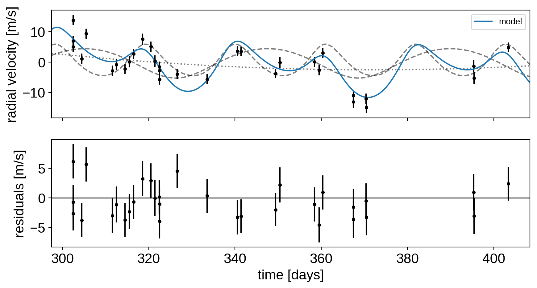
That looks pretty similar to what we got in Radial velocity fitting. Now let’s also plot the transit model.
def plot_light_curve(soln, mask=None):
    if mask is None:
        mask = np.ones(len(x), dtype=bool)

    fig, axes = plt.subplots(3, 1, figsize=(10, 7), sharex=True)

    ax = axes[0]
    ax.plot(x[mask], y[mask], "k", label="data")
    gp_mod = soln["gp_pred"] + soln["mean"]
    ax.plot(x[mask], gp_mod, color="C2", label="gp model")
    ax.legend(fontsize=10)
    ax.set_ylabel("relative flux [ppt]")

    ax = axes[1]
    ax.plot(x[mask], y[mask] - gp_mod, "k", label="de-trended data")
    for i, l in enumerate("bc"):
        mod = soln["light_curves"][:, i]
        ax.plot(x[mask], mod, label="planet {0}".format(l))
    ax.legend(fontsize=10, loc=3)
    ax.set_ylabel("de-trended flux [ppt]")

    ax = axes[2]
    mod = gp_mod + np.sum(soln["light_curves"], axis=-1)
    ax.plot(x[mask], y[mask] - mod, "k")
    ax.axhline(0, color="#aaaaaa", lw=1)
    ax.set_ylabel("residuals [ppt]")
    ax.set_xlim(x[mask].min(), x[mask].max())
    ax.set_xlabel("time [days]")

    return fig

plot_light_curve(map_soln0);
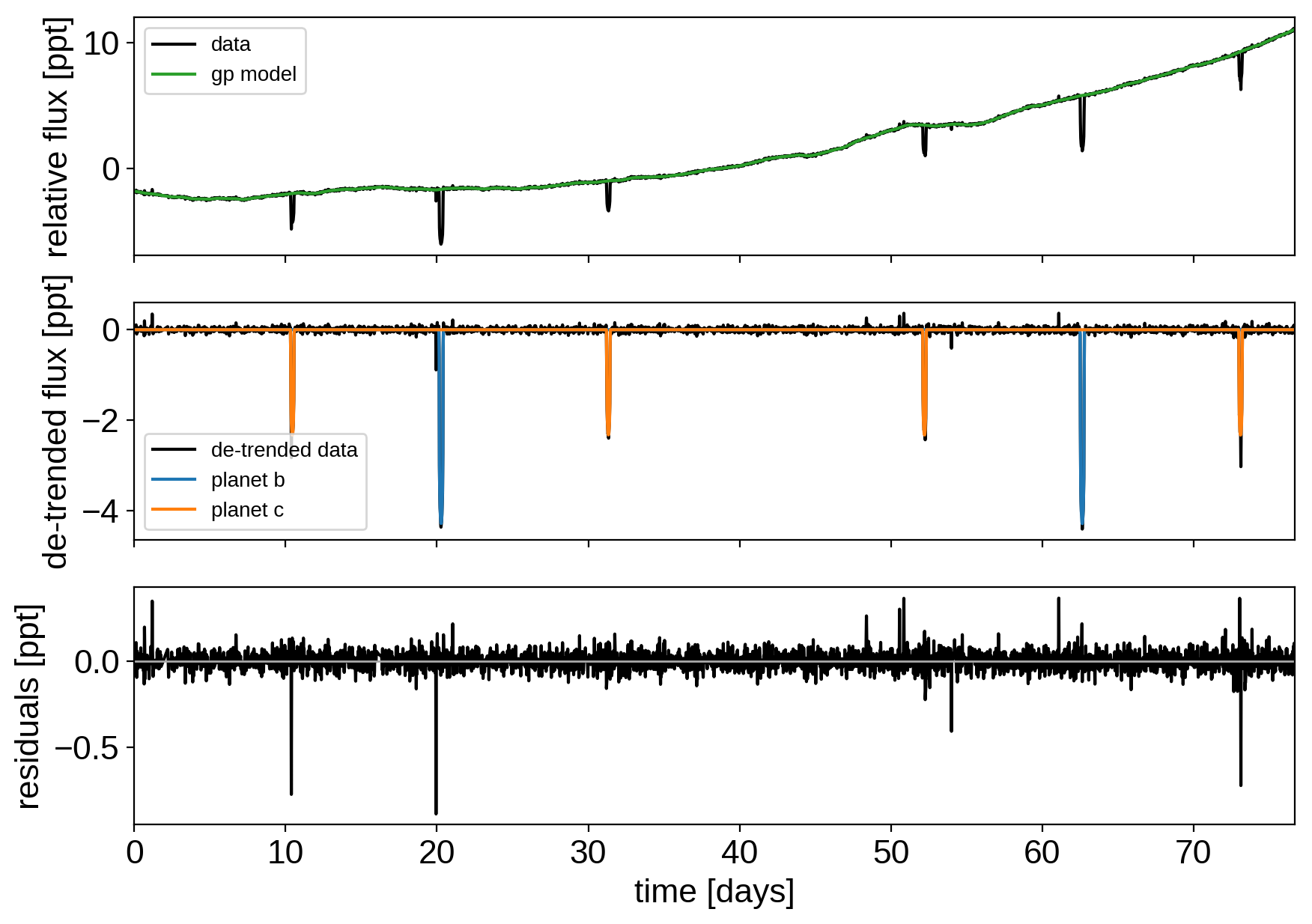
There are still a few outliers in the light curve and it can be useful to remove those before doing the full fit because both the GP and transit parameters can be sensitive to this.
To remove the outliers, we’ll look at the empirical RMS of the residuals away from the GP + transit model and remove anything that is more than a 7-sigma outlier.
mod = map_soln0["gp_pred"] + map_soln0["mean"] + np.sum(map_soln0["light_curves"], axis=-1)
resid = y - mod
rms = np.sqrt(np.median(resid**2))
mask = np.abs(resid) < 7 * rms

plt.plot(x, resid, "k", label="data")
plt.plot(x[~mask], resid[~mask], "xr", label="outliers")
plt.axhline(0, color="#aaaaaa", lw=1)
plt.ylabel("residuals [ppt]")
plt.xlabel("time [days]")
plt.legend(fontsize=12, loc=4)
plt.xlim(x.min(), x.max());
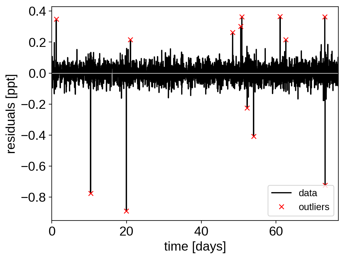
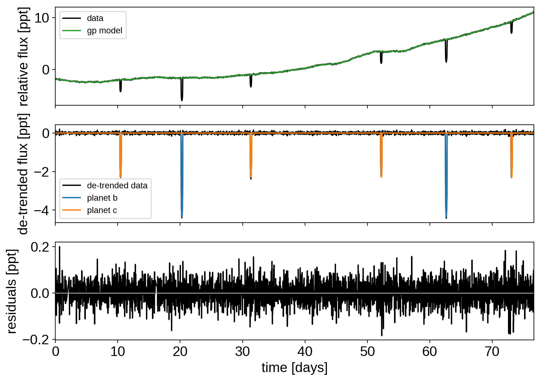
That looks better. Let’s re-build our model with this sigma-clipped dataset.
model, map_soln = build_model(mask, map_soln0)
plot_light_curve(map_soln, mask);
optimizing logp for variables: [trend]
6it [00:01,  3.87it/s, logp=5.225381e+03]
message: Desired error not necessarily achieved due to precision loss.
logp: 5225.3812218700705 -> 5225.3812218700705
optimizing logp for variables: [logs2]
9it [00:01,  5.64it/s, logp=5.307429e+03]
message: Optimization terminated successfully.
logp: 5225.3812218700705 -> 5307.429388952928
optimizing logp for variables: [b, logr, r_star]
85it [00:01, 53.15it/s, logp=5.318396e+03]
message: Desired error not necessarily achieved due to precision loss.
logp: 5307.429388952928 -> 5318.395980443081
optimizing logp for variables: [t0, logP]
109it [00:01, 57.38it/s, logp=5.319775e+03]
message: Desired error not necessarily achieved due to precision loss.
logp: 5318.395980443073 -> 5319.775397564113
optimizing logp for variables: [logSw4, logs2]
10it [00:01,  5.26it/s, logp=5.320504e+03]
message: Optimization terminated successfully.
logp: 5319.775397564102 -> 5320.504272670553
optimizing logp for variables: [logw0]
9it [00:01,  6.25it/s, logp=5.320538e+03]
message: Optimization terminated successfully.
logp: 5320.504272670553 -> 5320.538334045068
optimizing logp for variables: [logSw4, logw0, logs2, trend, logs_rv, omega, ecc_frac, ecc_sigma_rayleigh, ecc_sigma_gauss, ecc, b, logr, t0, logP, logm, r_star, m_star, u_star, mean]
156it [00:02, 56.51it/s, logp=5.322099e+03]
message: Desired error not necessarily achieved due to precision loss.
logp: 5320.538334045072 -> 5322.099130377849
Great! Now we’re ready to sample.
The sampling for this model is the same as for all the previous tutorials, but it takes a bit longer (about 2 hours on my laptop). This is partly because the model is more expensive to compute than the previous ones and partly because there are some non-affine degeneracies in the problem (for example between impact parameter and eccentricity). It might be worth thinking about reparameterizations (in terms of duration instead of eccentricity), but that’s beyond the scope of this tutorial. Besides, using more traditional MCMC methods, this would have taken a lot more than 2 hours to get >1000 effective samples!
np.random.seed(123)
with model:
    trace = pm.sample(tune=6000, draws=3000, start=map_soln, chains=4,
                      step=xo.get_dense_nuts_step(target_accept=0.9))
Multiprocess sampling (4 chains in 4 jobs)
NUTS: [logSw4, logw0, logs2, trend, logs_rv, omega, ecc_frac, ecc_sigma_rayleigh, ecc_sigma_gauss, ecc, b, logr, t0, logP, logm, r_star, m_star, u_star, mean]
Sampling 4 chains: 100%|██████████| 36000/36000 [1:10:28<00:00,  2.63draws/s]
There were 50 divergences after tuning. Increase target_accept or reparameterize.
There were 28 divergences after tuning. Increase target_accept or reparameterize.
There were 68 divergences after tuning. Increase target_accept or reparameterize.
There were 28 divergences after tuning. Increase target_accept or reparameterize.
The number of effective samples is smaller than 10% for some parameters.
Let’s look at the convergence diagnostics for some of the key parameters:
pm.summary(trace, varnames=["period", "r_pl", "m_pl", "ecc", "omega", "b"])
| mean | sd | mc_error | hpd_2.5 | hpd_97.5 | n_eff | Rhat | |
|---|---|---|---|---|---|---|---|
| period__0 | 42.363463 | 0.000392 | 0.000004 | 42.362708 | 42.364246 | 9151.208199 | 0.999957 |
| period__1 | 20.885336 | 0.000203 | 0.000002 | 20.884935 | 20.885732 | 10604.924899 | 0.999950 |
| r_pl__0 | 0.077460 | 0.004526 | 0.000120 | 0.068487 | 0.086384 | 1420.136330 | 1.000589 |
| r_pl__1 | 0.055808 | 0.003547 | 0.000099 | 0.048599 | 0.062616 | 1303.025125 | 1.000549 |
| m_pl__0 | 27.211132 | 5.982638 | 0.081521 | 15.826499 | 39.414731 | 5703.290722 | 1.000004 |
| m_pl__1 | 22.131311 | 4.337161 | 0.045731 | 13.411342 | 30.572525 | 7589.478890 | 0.999873 |
| ecc__0 | 0.038365 | 0.034152 | 0.000638 | 0.000002 | 0.105034 | 3089.089741 | 0.999993 |
| ecc__1 | 0.104319 | 0.090297 | 0.002147 | 0.000020 | 0.283987 | 1601.006227 | 1.000687 |
| omega__0 | 0.175756 | 2.002201 | 0.032419 | -2.920794 | 3.136844 | 3214.012068 | 1.000786 |
| omega__1 | -0.348717 | 1.037055 | 0.020597 | -2.637688 | 2.106129 | 2440.620305 | 1.000854 |
| b__0 | 0.588610 | 0.049182 | 0.001265 | 0.490307 | 0.667716 | 1594.169568 | 1.001262 |
| b__1 | 0.532838 | 0.122761 | 0.004287 | 0.280008 | 0.726690 | 790.467593 | 1.001656 |
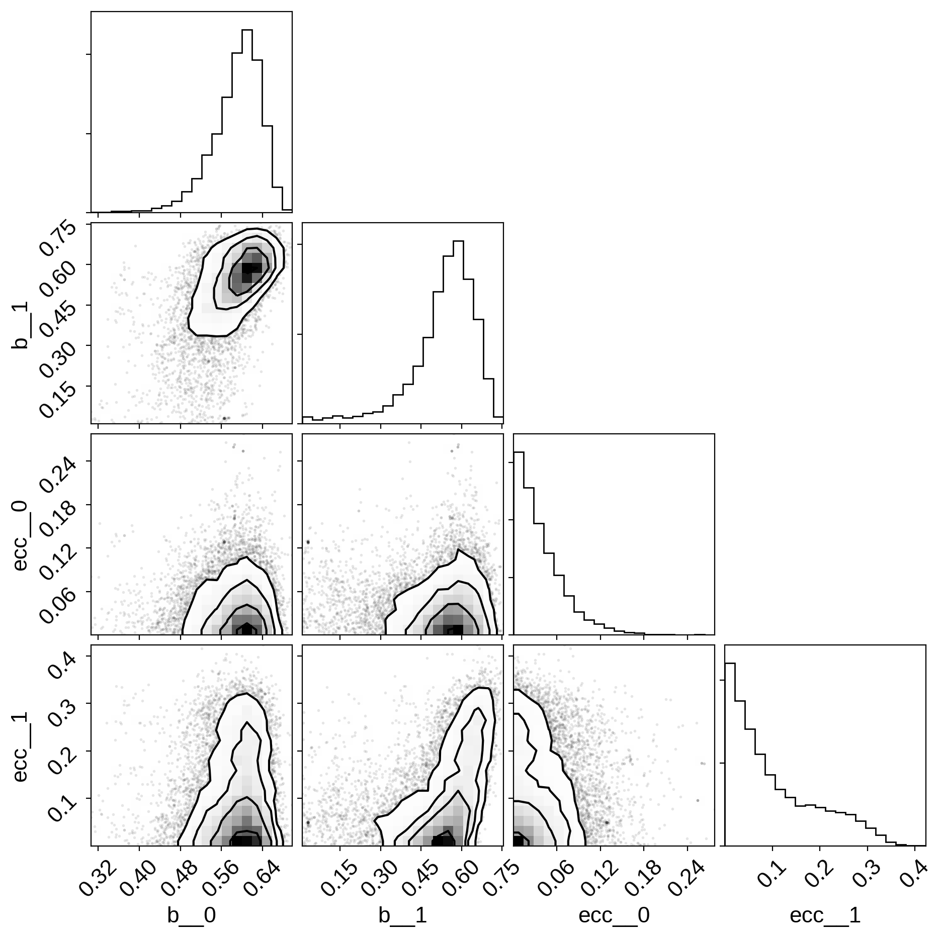
As you see, the effective number of samples for the impact parameters and eccentricites are lower than for the other parameters. This is because of the correlations that I mentioned above:
import corner
varnames = ["b", "ecc"]
samples = pm.trace_to_dataframe(trace, varnames=varnames)
fig = corner.corner(samples);
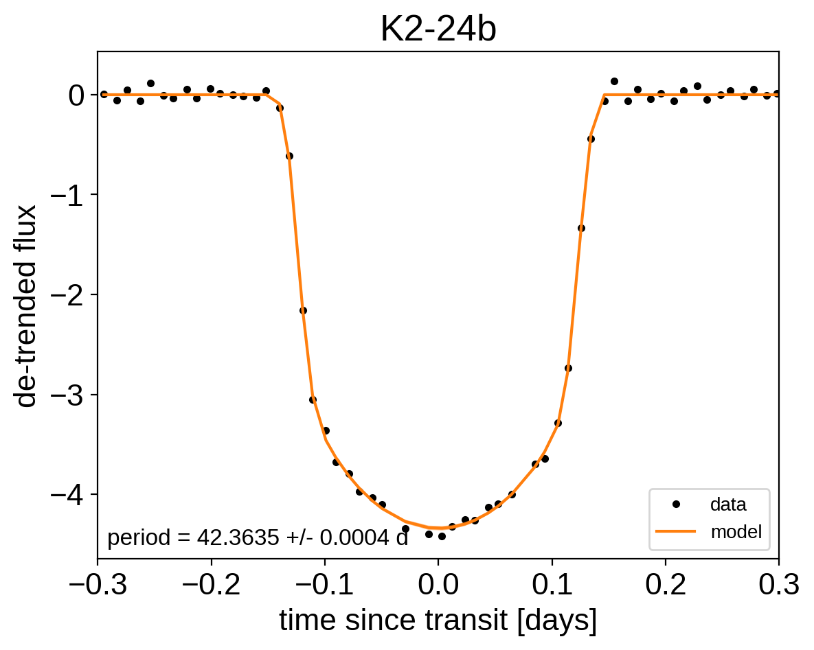
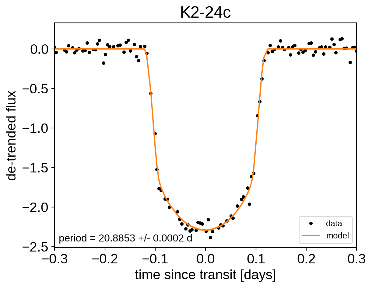
Finally, as in the Radial velocity fitting and Transit fitting tutorials, we can make folded plots of the transits and the radial velocities and compare to the posterior model predictions. (Note: planets b and c in this tutorial are swapped compared to the labels from Petigura et al. (2016))
for n, letter in enumerate("bc"):
    plt.figure()

    # Compute the GP prediction
    gp_mod = np.median(trace["gp_pred"] + trace["mean"][:, None], axis=0)

    # Get the posterior median orbital parameters
    p = np.median(trace["period"][:, n])
    t0 = np.median(trace["t0"][:, n])

    # Compute the median of posterior estimate of the contribution from
    # the other planet. Then we can remove this from the data to plot
    # just the planet we care about.
    other = np.median(trace["light_curves"][:, :, (n + 1) % 2], axis=0)

    # Plot the folded data
    x_fold = (x[mask] - t0 + 0.5*p) % p - 0.5*p
    plt.plot(x_fold, y[mask] - gp_mod - other, ".k", label="data", zorder=-1000)

    # Plot the folded model
    inds = np.argsort(x_fold)
    inds = inds[np.abs(x_fold)[inds] < 0.3]
    pred = trace["light_curves"][:, inds, n]
    pred = np.percentile(pred, [16, 50, 84], axis=0)
    plt.plot(x_fold[inds], pred[1], color="C1", label="model")
    art = plt.fill_between(x_fold[inds], pred[0], pred[2], color="C1", alpha=0.5,
                           zorder=1000)
    art.set_edgecolor("none")

    # Annotate the plot with the planet's period
    txt = "period = {0:.4f} +/- {1:.4f} d".format(
        np.mean(trace["period"][:, n]), np.std(trace["period"][:, n]))
    plt.annotate(txt, (0, 0), xycoords="axes fraction",
                 xytext=(5, 5), textcoords="offset points",
                 ha="left", va="bottom", fontsize=12)

    plt.legend(fontsize=10, loc=4)
    plt.xlim(-0.5*p, 0.5*p)
    plt.xlabel("time since transit [days]")
    plt.ylabel("de-trended flux")
    plt.title("K2-24{0}".format(letter));
    plt.xlim(-0.3, 0.3)
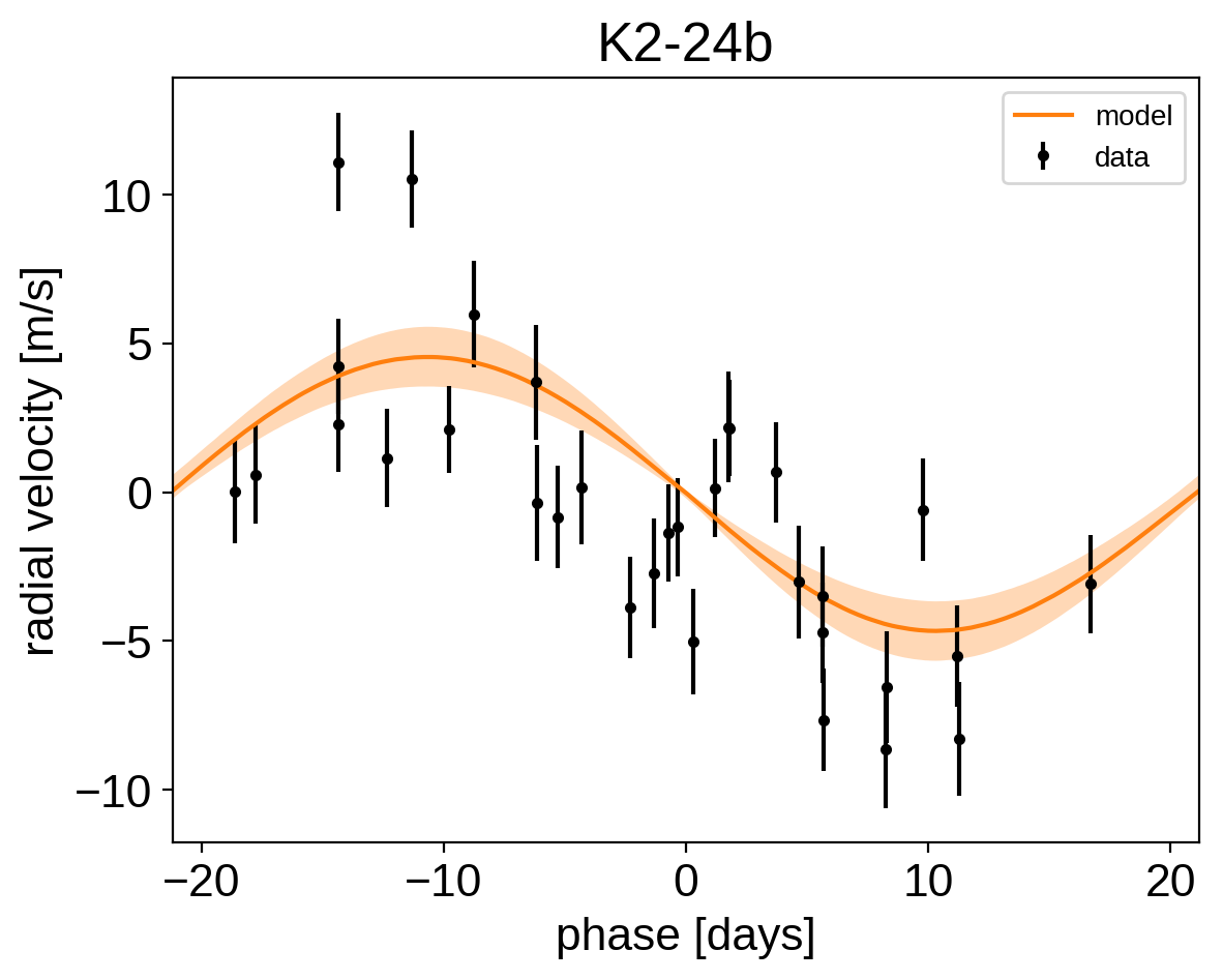
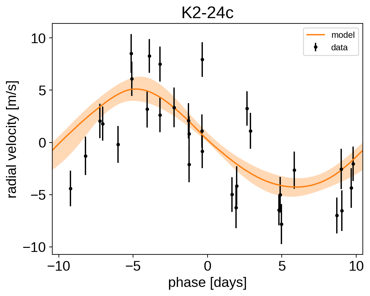
for n, letter in enumerate("bc"):
    plt.figure()

    # Get the posterior median orbital parameters
    p = np.median(trace["period"][:, n])
    t0 = np.median(trace["t0"][:, n])

    # Compute the median of posterior estimate of the background RV
    # and the contribution from the other planet. Then we can remove
    # this from the data to plot just the planet we care about.
    other = np.median(trace["vrad"][:, :, (n + 1) % 2], axis=0)
    other += np.median(trace["bkg"], axis=0)

    # Plot the folded data
    x_fold = (x_rv - t0 + 0.5*p) % p - 0.5*p
    plt.errorbar(x_fold, y_rv - other, yerr=yerr_rv, fmt=".k", label="data")

    # Compute the posterior prediction for the folded RV model for this
    # planet
    t_fold = (t_rv - t0 + 0.5*p) % p - 0.5*p
    inds = np.argsort(t_fold)
    pred = np.percentile(trace["vrad_pred"][:, inds, n], [16, 50, 84], axis=0)
    plt.plot(t_fold[inds], pred[1], color="C1", label="model")
    art = plt.fill_between(t_fold[inds], pred[0], pred[2], color="C1", alpha=0.3)
    art.set_edgecolor("none")

    plt.legend(fontsize=10)
    plt.xlim(-0.5*p, 0.5*p)
    plt.xlabel("phase [days]")
    plt.ylabel("radial velocity [m/s]")
    plt.title("K2-24{0}".format(letter));
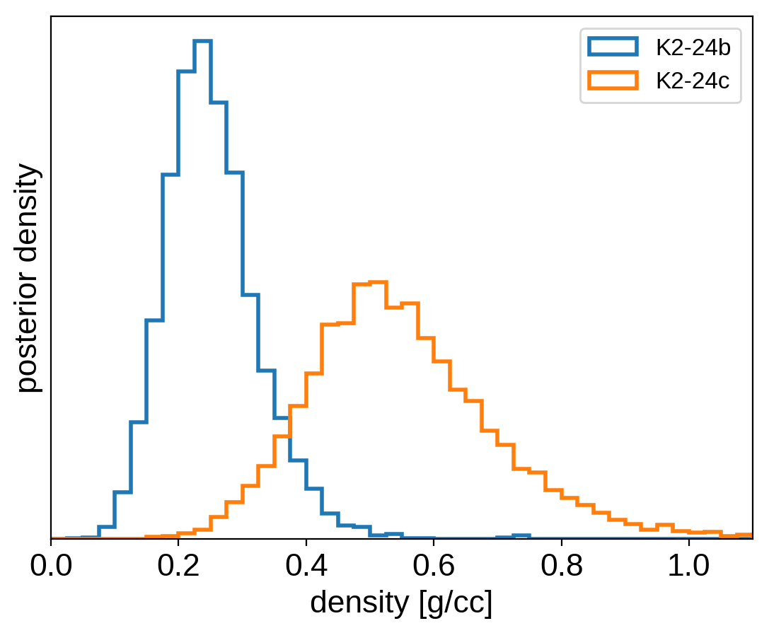
We can also compute the posterior constraints on the planet densities.
volume = 4/3*np.pi*trace["r_pl"]**3
density = u.Quantity(trace["m_pl"] / volume, unit=u.M_earth / u.R_sun**3)
density = density.to(u.g / u.cm**3).value

bins = np.linspace(0, 1.1, 45)
for n, letter in enumerate("bc"):
    plt.hist(density[:, n], bins, histtype="step", lw=2,
             label="K2-24{0}".format(letter), density=True)
plt.yticks([])
plt.legend(fontsize=12)
plt.xlim(bins[0], bins[-1])
plt.xlabel("density [g/cc]")
plt.ylabel("posterior density");
As described in the Citing exoplanet & its dependencies tutorial, we can use
exoplanet.citations.get_citations_for_model() to construct an
acknowledgement and BibTeX listing that includes the relevant citations
for this model.
with model:
    txt, bib = xo.citations.get_citations_for_model()
print(txt)
This research made use of textsf{exoplanet} citep{exoplanet} and its
dependencies citep{exoplanet:agol19, exoplanet:astropy13, exoplanet:astropy18,
exoplanet:exoplanet, exoplanet:foremanmackey17, exoplanet:foremanmackey18,
exoplanet:kipping13, exoplanet:luger18, exoplanet:pymc3, exoplanet:theano,
exoplanet:vaneylen19}.
print("\n".join(bib.splitlines()[:10]) + "\n...")
@misc{exoplanet:exoplanet,
  author = {Daniel Foreman-Mackey and Ian Czekala and Eric Agol and
            Rodrigo Luger and Geert Barentsen and Tom Barclay},
   title = {dfm/exoplanet: exoplanet v0.2.0},
   month = aug,
    year = 2019,
     doi = {10.5281/zenodo.3359880},
     url = {https://doi.org/10.5281/zenodo.3359880}
}
...