Automatic differentation & gradient-based inference

import exoplanet

exoplanet.utils.docs_setup()
print(f"exoplanet.__version__ = '{exoplanet.__version__}'")

WARNING (theano.tensor.blas): Using NumPy C-API based implementation for BLAS functions.

exoplanet.__version__ = '0.5.4.dev0+g4fd768a.d20221013'

The major selling point of exoplanet compared to other similar libraries is that it integrates with the PyMC3 probabilistic modeling framework. PyMC3 offers gradient-based inference algorithms (more on these below) that can be more computationally efficient (per effective sample) than other tools commonly used for probabilistic inference in astrophysics. When I am writing this, gradient-based inference methodology is not widely used in astro because it can be difficult to compute the relevant gradients (derivatives of your log probability function with respect to the parameters). PyMC3 (and many other frameworks like it) handle this issue using automatic differentiation (AD), a method (or collection of methods) for automatically propagating derivatives through your code.

It’s beyond the scope of this tutorial to go into too many details about AD and most users of exoplanet shouldn’t need to interact with this too much, but this should at least give you a little taste of the kinds of things AD can do for you and demonstrate how this translates into efficient inference with probabilistic models. The main thing that I want to emphasize here is that AD is not the same as symbolic differentiation (it’s not going to provide you with a mathematical expression for your gradients), but it’s also not the same as numerical methods like finite difference. Using AD to evaluate the gradients of your model will generally be faster, more efficient, and more numerically stable than alternatives, but there are always exceptions to any rule. There are times when providing your AD framework with a custom implementation and/or differentation rule for a particular function is beneficial in terms of cost and stability. exoplanet is designed to provide these custom implementations only where it is useful (e.g. solving Kepler’s equation or evaluating limb-darkened light curves) and then rely on the existing AD toolkit elsewhere.

Automatic differentation in Theano/Aesara

Let’s start by giving a quick taste for how AD works in the context of PyMC3 and exoplanet. PyMC3 is built on top of a library called Aesara (formerly Theano, see Theano vs. Aesara) that was designed for AD and fast linear algebra in the context of neural networks. The learning curve can be steep because your code ends up looking a little different from the usual way you would write Python code. (If you’re looking for something more “Pythonic”, JAX might be a good alternative, but for our purposes we’ll stick with Aesara.) In Aesara, you start be defining the relationships between variables and then ask to evaluate a variable using this “graph”. This might seem a little counterintuitive and you hopefully won’t have to worry about this too much, but it can be a handy workflow because Aesara will compile and optimize your model in the background (generally making it faster). This structure allows us to evaluate the derivative of some variable with respect to another.

Here’s a simple example where we define a relationship between two variables x and y:

\[ y = \exp\left[\sin\left(\frac{2\,\pi\,x}{3}\right)\right] \]

and then calculate the derivative using AD. For comparison, the symbolic derivative is:

\[ \frac{\mathrm{d}y}{\mathrm{d}x} = \frac{2\,\pi}{3}\,\exp\left[\sin\left(\frac{2\,\pi\,x}{3}\right)\right]\,\cos\left(\frac{2\,\pi\,x}{3}\right) \]

import numpy as np
import matplotlib.pyplot as plt
from aesara_theano_fallback import aesara
import aesara_theano_fallback.tensor as at

# Define the relationship between two variables x and y=f(x)
x_ = at.vector("x")
y_ = at.exp(at.sin(2 * np.pi * x_ / 3.0))

# Here aesara will compile a function to evaluate y
func = aesara.function([x_], y_)

# Request the gradient of y with respect to x
# Note the call to `sum`. This is a bit of a cheat since by
# default Aesara only computes gradients of a *scalar* function
grad = aesara.function([x_], aesara.grad(at.sum(y_), x_))

# Plot the function and its derivative
x = np.linspace(-3, 3, 500)
plt.plot(x, func(x), "k", lw=1, label="f(x)")
plt.plot(x, grad(x), "C0", label="df(x)/dx; AD", lw=3)

# Overplot the symbolic derivative for comparison
plt.plot(
    x,
    2 * np.pi * func(x) * np.cos(2 * np.pi * x / 3.0) / 3.0,
    "C1",
    lw=1,
    label="df(x)/dx; symbolic",
)

plt.legend()
plt.title("a silly function and its derivative")
plt.ylabel("f(x); df(x)/dx")
_ = plt.xlabel("x")

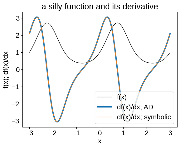
This example is obviously pretty artificial, but I think that you can imagine how something like this would start to come in handy when your models get more complicated. In particular, I think that you’ll probably pretty regularly find yourself experimenting with different choices of parameters and it would be a real pain to be required to re-write all your derivative code for every new choice of parameterization.

Gradient-based inference

Now that we have a way of easily evaluating the derivatives of scalar functions, we have a wide array of new inference algorithms at our disposal. For example, if we use Aesara to evaluate our log probability function, we could pass the value and gradient to scipy.optimize.minimize in order to find the maximum likelihood or maximum a posteriori parameters. But, the point of exoplanet is that it integrates with PyMC3 which provides implementations of various gradient-based Markov chain Monte Carlo (MCMC) methods like Hamiltonian Monte Carlo and No U-Turn Sampling. PyMC3 also supports gradient-based methods for variational inference, but (so far) exoplanet had mostly been used for MCMC.

Take a look at A quick intro to PyMC3 for some specific introductory examples of using PyMC3 for MCMC, but the general motivation for using PyMC3 (instead of emcee or dynesty, for example) is that it can be far more computationally efficient (per effective sample), especially when your model has more than a couple of parameters. We’re not going to do a systematic study of the relative performance of different methods because that is fraught and can be problem specific, but let’s look at another very artificial example where we compare the performance of sampling a 50-dimensional Gaussian using PyMC3 and emcee.

import time
import emcee
import logging
import pymc3 as pm
import arviz as az
import pymc3_ext as pmx

# Make PyMC3 less noisy just for this example!
logger = logging.getLogger("pymc3")
logger.setLevel(logging.ERROR)

# First define and sample the model using PyMC3
with pm.Model() as model:
    pm.Normal("x", shape=50)

    # Run a fake chain just to get everything to compile
    pm.sample(
        tune=1, draws=1, chains=1, return_inferencedata=True, progressbar=False
    )

    # Run and time the sampling
    start = time.time()
    pymc_trace = pm.sample(
        tune=1000,
        draws=1000,
        chains=2,
        cores=1,
        return_inferencedata=True,
        progressbar=False,
    )
    pymc_time = time.time() - start

    # Compute the cost per sample
    pymc_per_eff = pymc_time / np.mean(az.summary(pymc_trace)["ess_bulk"])

# Then sample the same model using emcee
func = pmx.get_theano_function_for_var(model.logpt, model=model)


def logp(theta):
    return func(theta)


init = np.random.randn(124, model.ndim)
nwalkers, ndim = init.shape
sampler = emcee.EnsembleSampler(nwalkers, ndim, logp)

start = time.time()
init = sampler.run_mcmc(init, 1000)
sampler.reset()
sampler.run_mcmc(init, 3000)
emcee_time = time.time() - start

emcee_trace = az.from_emcee(sampler=sampler)
emcee_per_eff = emcee_time / np.mean(az.summary(emcee_trace)["ess_bulk"])

After running these chains, we can compare the relative performance (remember that this is a very artificial example so caveats, small print, yadda, etc.). To compare the performance of different MCMC samplers, the best metric is the computational cost per effective sample (for the parameter/function that you most care about). In this case, we’ll look at the total runtime (including burn-in) divided by an estaimte of the the mean effective sample size across all 50 dimensions (lower is better):

print(
    f"For PyMC3, the runtime per effective sample is: {pymc_per_eff * 1e3:.2f} ms"
)
print(
    f"For emcee, the runtime per effective sample is: {emcee_per_eff * 1e3:.2f} ms"
)

For PyMC3, the runtime per effective sample is: 0.65 ms
For emcee, the runtime per effective sample is: 33.73 ms

So, in this case, PyMC3 is a few order of magnitude more efficient. As your models get more complex (in terms of computational cost, number of parameters, and the geometry of your parameter space), your mileage might vary, but my experience is that using PyMC3 is almost always a good idea if you can!

Tip

If you find that your model is not sampling well, this is almost always caused by parameterization issues and you’ll probably get drastically better performance with some reparameterization. See Reparameterization for some tips and tricks.