Note

This tutorial was generated from an IPython notebook that can be downloaded here.

Transit fitting¶

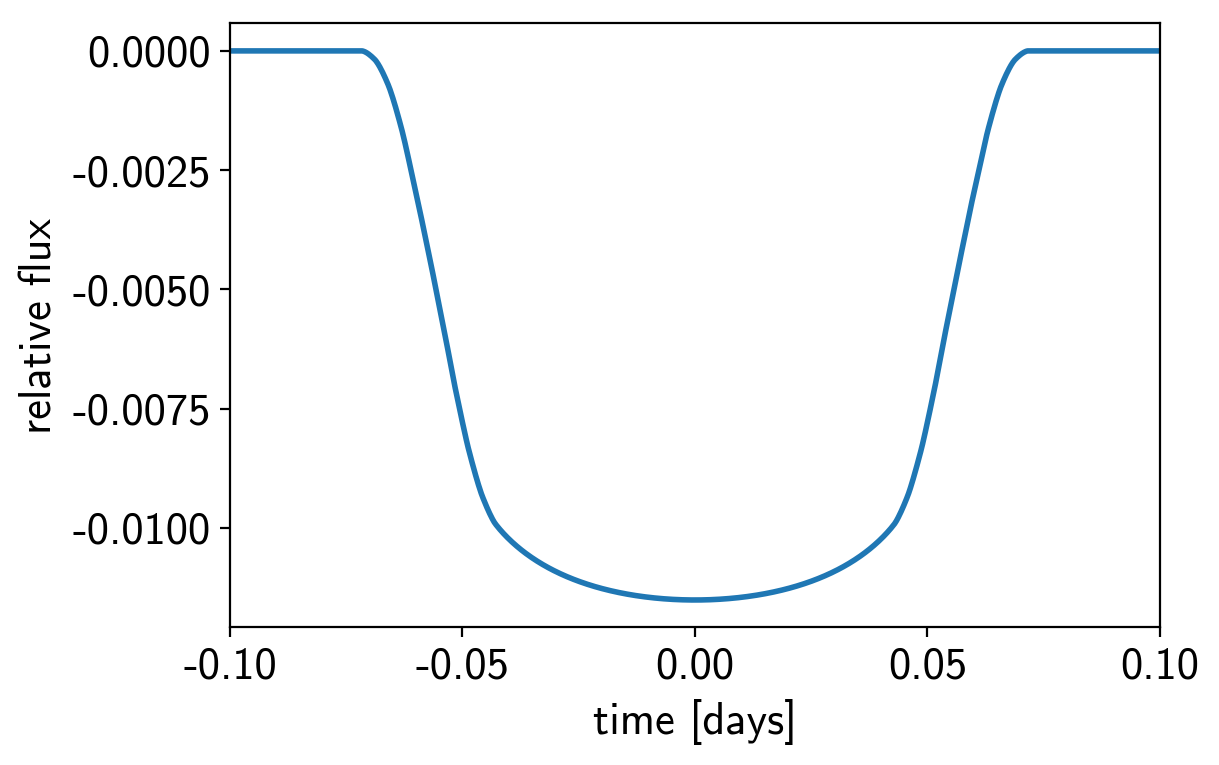
exoplanet includes methods for computing the light curves transiting planets. In its simplest form this can be used to evaluate a light curve like you would do with batman, for example:

import numpy as np
import matplotlib.pyplot as plt

import exoplanet as xo

# The light curve calculation requires an orbit
orbit = xo.orbits.KeplerianOrbit(period=3.456)

# Compute a limb-darkened light curve using starry
t = np.linspace(-0.1, 0.1, 1000)
u = [0.3, 0.2]
light_curve = xo.StarryLightCurve(u).get_light_curve(
    orbit=orbit, r=0.1, t=t, texp=0.02).eval()
# Note: the `eval` is needed because this is using Theano in
# the background

plt.plot(t, light_curve, color="C0", lw=2)
plt.ylabel("relative flux")
plt.xlabel("time [days]")
plt.xlim(t.min(), t.max());

But the real power comes from the fact that this is defined as a Theano operation so it can be combined with PyMC3 to do transit inference using Hamiltonian Monte Carlo.

The transit model in PyMC3¶

In this section, we will construct a simple transit fit model using PyMC3 and then we will fit a two planet model to simulated data. To start, let’s randomly sample some periods and phases and then define the time sampling:

np.random.seed(123)
periods = np.random.uniform(5, 20, 2)
t0s = periods * np.random.rand(2)
t = np.arange(0, 80, 0.02)
yerr = 5e-4

Then, define the parameters. In this simple model, we’ll just fit for the limb darkening parameters of the star, and the period, phase, impact parameter, and radius ratio of the planets (note: this is already 10 parameters and running MCMC to convergence using emcee would probably take at least an hour). For the limb darkening, we’ll use a quadratic law as parameterized by Kipping (2013) and for the joint radius ratio and impact parameter distribution we’ll use the parameterization from Espinoza (2018). Both of these reparameterizations are implemented in exoplanet as custom PyMC3 distributions (exoplanet.distributions.QuadLimbDark and exoplanet.distributions.RadiusImpact respectively).

import pymc3 as pm

with pm.Model() as model:

    # The baseline flux
    mean = pm.Normal("mean", mu=0.0, sd=1.0)

    # The time of a reference transit for each planet
    t0 = pm.Normal("t0", mu=t0s, sd=1.0, shape=2)

    # The log period; also tracking the period itself
    logP = pm.Normal("logP", mu=np.log(periods), sd=0.1, shape=2)
    period = pm.Deterministic("period", pm.math.exp(logP))

    # The Kipping (2013) parameterization for quadratic limb darkening paramters
    u = xo.distributions.QuadLimbDark("u", testval=np.array([0.3, 0.2]))

    # The Espinoza (2018) parameterization for the joint radius ratio and
    # impact parameter distribution
    r, b = xo.distributions.get_joint_radius_impact(
        min_radius=0.01, max_radius=0.1,
        testval_r=np.array([0.04, 0.06]),
        testval_b=np.random.rand(2)
    )

    # This shouldn't make a huge difference, but I like to put a uniform
    # prior on the *log* of the radius ratio instead of the value. This
    # can be implemented by adding a custom "potential" (log probability).
    pm.Potential("r_prior", -pm.math.log(r))

    # Set up a Keplerian orbit for the planets
    orbit = xo.orbits.KeplerianOrbit(period=period, t0=t0, b=b)

    # Compute the model light curve using starry
    light_curves = xo.StarryLightCurve(u).get_light_curve(
        orbit=orbit, r=r, t=t)
    light_curve = pm.math.sum(light_curves, axis=-1) + mean

    # Here we track the value of the model light curve for plotting
    # purposes
    pm.Deterministic("light_curves", light_curves)

    # In this line, we simulate the dataset that we will fit
    y = xo.eval_in_model(light_curve)
    y += yerr * np.random.randn(len(y))

    # The likelihood function assuming known Gaussian uncertainty
    pm.Normal("obs", mu=light_curve, sd=yerr, observed=y)

    # Fit for the maximum a posteriori parameters given the simuated
    # dataset
    map_soln = pm.find_MAP(start=model.test_point)

logp = 24,806, ||grad|| = 2,665.9: 100%|██████████| 24/24 [00:00<00:00, 506.80it/s]

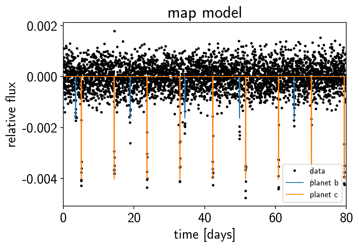
Now we can plot the simulated data and the maximum a posteriori model to make sure that our initialization looks ok.

plt.plot(t, y, ".k", ms=4, label="data")
for i, l in enumerate("bc"):
    plt.plot(t, map_soln["light_curves"][:, i], lw=1,
             label="planet {0}".format(l))
plt.xlim(t.min(), t.max())
plt.ylabel("relative flux")
plt.xlabel("time [days]")
plt.legend(fontsize=10)
plt.title("map model");

Sampling¶

Now, let’s sample from the posterior defined by this model. As usual, there are strong covariances between some of the parameters so we’ll use the exoplanet.PyMC3Sampler to sample.

np.random.seed(42)
sampler = xo.PyMC3Sampler(window=100, finish=200)
with model:
    burnin = sampler.tune(tune=2500, start=map_soln, step_kwargs=dict(target_accept=0.9))
    trace = sampler.sample(draws=3000)

Sampling 4 chains: 100%|██████████| 308/308 [00:13<00:00, 23.38draws/s]
Sampling 4 chains: 100%|██████████| 408/408 [00:18<00:00, 22.01draws/s]
Sampling 4 chains: 100%|██████████| 808/808 [00:29<00:00, 27.40draws/s]
Sampling 4 chains: 100%|██████████| 1608/1608 [00:05<00:00, 268.51draws/s]
Sampling 4 chains: 100%|██████████| 6908/6908 [00:22<00:00, 313.50draws/s]
Multiprocess sampling (4 chains in 4 jobs)
NUTS: [rb, u, logP, t0, mean]
Sampling 4 chains: 100%|██████████| 12800/12800 [00:40<00:00, 312.34draws/s]

After sampling, it’s important that we assess convergence. We can do that using the pymc3.summary function:

pm.summary(trace, varnames=["period", "t0", "r", "b", "u", "mean"])

	mean	sd	mc_error	hpd_2.5	hpd_97.5	n_eff	Rhat
period__0	15.447923	0.002286	3.203097e-05	15.443245	15.452077	4254.978576	0.999958
period__1	9.292480	0.000299	2.672398e-06	9.291904	9.293061	11308.907964	0.999891
t0__0	3.503033	0.005793	8.547461e-05	3.492053	3.514400	4091.199571	1.000061
t0__1	5.121266	0.001344	1.167547e-05	5.118695	5.123957	14160.384039	0.999856
r__0	0.039527	0.001599	2.003953e-05	0.036392	0.042555	6474.021735	0.999977
r__1	0.058460	0.001048	1.442094e-05	0.056406	0.060387	5641.558519	1.000176
b__0	0.668798	0.047877	8.287093e-04	0.568748	0.741457	3823.304052	0.999970
b__1	0.402672	0.038155	5.159546e-04	0.330739	0.471772	5394.376231	1.000179
u__0	0.369068	0.205079	1.979595e-03	0.000409	0.718908	9666.472812	1.000054
u__1	0.282218	0.337819	4.344555e-03	-0.319950	0.865346	6266.050324	1.000207
mean	0.000005	0.000008	5.855918e-08	-0.000010	0.000021	16618.423243	1.000117

That looks pretty good! Fitting this without exoplanet would have taken a lot more patience.

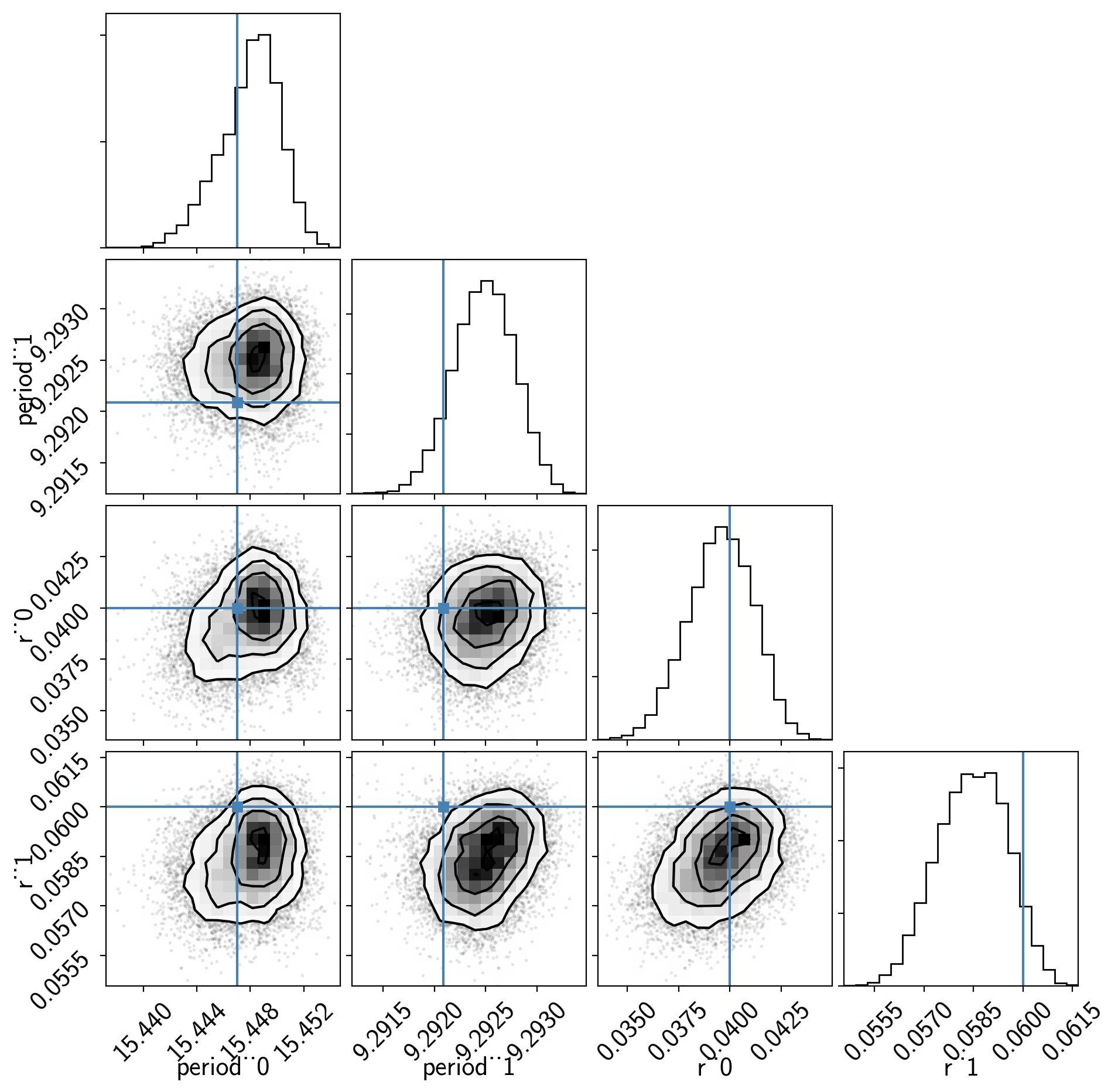
Now we can also look at the corner plot of some of that parameters of interest:

import corner
samples = pm.trace_to_dataframe(trace, varnames=["period", "r"])
truth = np.concatenate(xo.eval_in_model([period, r], model.test_point, model=model))
corner.corner(samples, truths=truth);

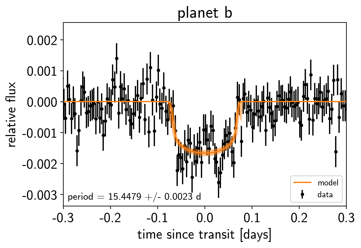
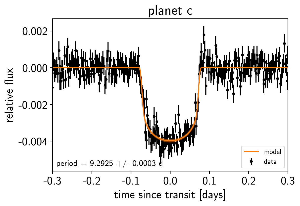
Phase plots¶

Like in the radial velocity tutorial (Radial velocity fitting), we can make plots of the model predictions for each planet.

for n, letter in enumerate("bc"):
    plt.figure()

    # Get the posterior median orbital parameters
    p = np.median(trace["period"][:, n])
    t0 = np.median(trace["t0"][:, n])

    # Compute the median of posterior estimate of the contribution from
    # the other planet. Then we can remove this from the data to plot
    # just the planet we care about.
    other = np.median(trace["light_curves"][:, :, (n + 1) % 2], axis=0)

    # Plot the folded data
    x_fold = (t - t0 + 0.5*p) % p - 0.5*p
    plt.errorbar(x_fold, y - other, yerr=yerr, fmt=".k", label="data",
                 zorder=-1000)

    # Plot the folded model
    inds = np.argsort(x_fold)
    inds = inds[np.abs(x_fold)[inds] < 0.3]
    pred = trace["light_curves"][:, inds, n] + trace["mean"][:, None]
    pred = np.percentile(pred, [16, 50, 84], axis=0)
    plt.plot(x_fold[inds], pred[1], color="C1", label="model")
    art = plt.fill_between(x_fold[inds], pred[0], pred[2], color="C1", alpha=0.5,
                           zorder=1000)
    art.set_edgecolor("none")

    # Annotate the plot with the planet's period
    txt = "period = {0:.4f} +/- {1:.4f} d".format(
        np.mean(trace["period"][:, n]), np.std(trace["period"][:, n]))
    plt.annotate(txt, (0, 0), xycoords="axes fraction",
                 xytext=(5, 5), textcoords="offset points",
                 ha="left", va="bottom", fontsize=12)

    plt.legend(fontsize=10, loc=4)
    plt.xlim(-0.5*p, 0.5*p)
    plt.xlabel("time since transit [days]")
    plt.ylabel("relative flux")
    plt.title("planet {0}".format(letter));
    plt.xlim(-0.3, 0.3)

Citations¶

As described in the Citing exoplanet & its dependencies tutorial, we can use exoplanet.citations.get_citations_for_model() to construct an acknowledgement and BibTeX listing that includes the relevant citations for this model. This is especially important here because we have used quite a few model components that should be cited.

with model:
    txt, bib = xo.citations.get_citations_for_model()
print(txt)

This research made use of textsf{exoplanet} citep{exoplanet} and its
dependencies citep{exoplanet:astropy13, exoplanet:astropy18,
exoplanet:espinoza18, exoplanet:exoplanet, exoplanet:kipping13,
exoplanet:luger18, exoplanet:pymc3, exoplanet:theano}.

print("\n".join(bib.splitlines()[:10]) + "\n...")

@misc{exoplanet:exoplanet,
    title={exoplanet v0.1.0},
   author={Foreman-Mackey, Daniel},
    month={dec},
     year={2018},
      doi={10.5281/zenodo.1998448},
      url={https://doi.org/10.5281/zenodo.1998448}
}

...

Transit fitting¶

The transit model in PyMC3¶

Sampling¶

Phase plots¶

Citations¶

Table Of Contents

Related Topics