Note
This tutorial was generated from an IPython notebook that can be downloaded here.
Case study: K2-24, putting it all together
theano version: 1.0.4
pymc3 version: 3.6
exoplanet version: 0.1.6
In this tutorial, we will combine many of the previous tutorials to perform a fit of the K2-24 system using the K2 transit data and the RVs from Petigura et al. (2016). This is the same system that we fit in the Radial velocity fitting tutorial and we’ll combine that model with the transit model from the Transit fitting tutorial and the Gaussian Process noise model from the Gaussian process models for stellar variability tutorial.
Datasets and initializations
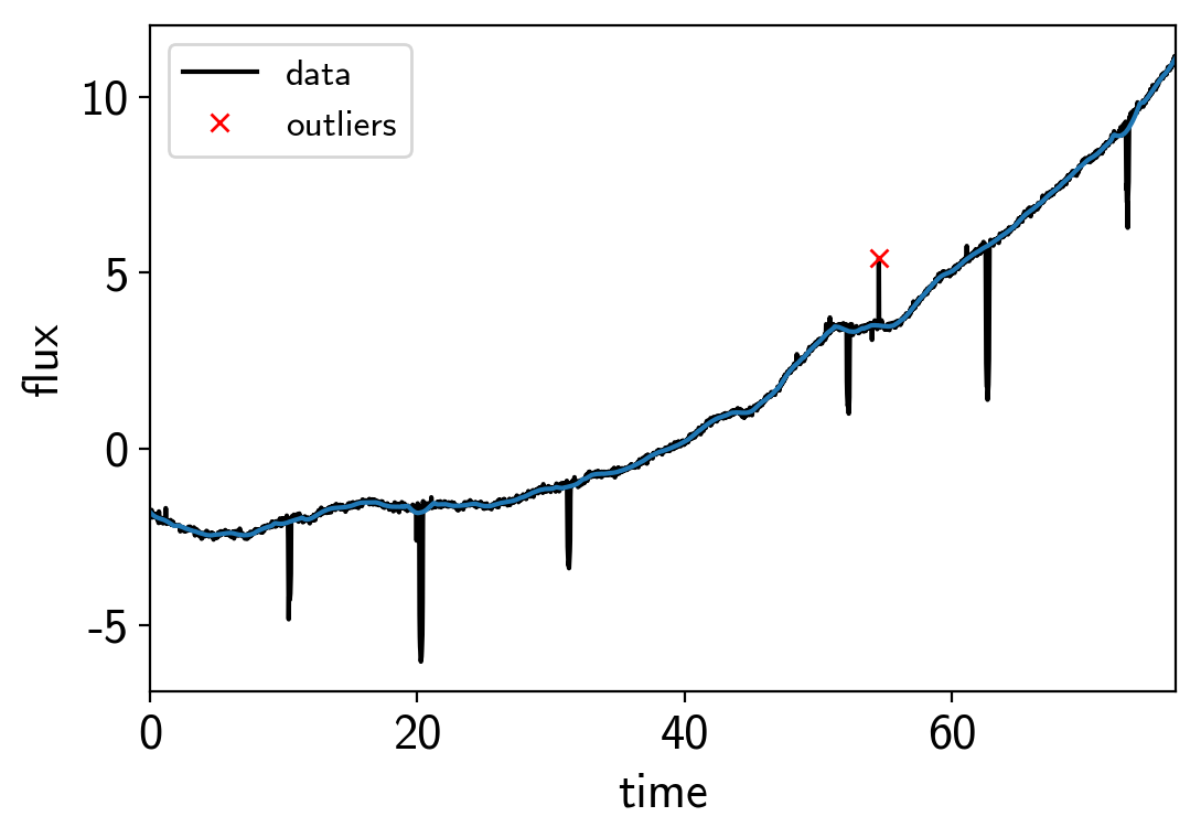
To get started, let’s download the relevant datasets. First, the transit light curve from Everest:
import numpy as np
import matplotlib.pyplot as plt

from astropy.io import fits
from scipy.signal import savgol_filter

# Download the data
lc_url = "https://archive.stsci.edu/hlsps/everest/v2/c02/203700000/71098/hlsp_everest_k2_llc_203771098-c02_kepler_v2.0_lc.fits"
with fits.open(lc_url) as hdus:
    lc = hdus[1].data
    lc_hdr = hdus[1].header

# Work out the exposure time
texp = lc_hdr["FRAMETIM"] * lc_hdr["NUM_FRM"]
texp /= 60.0 * 60.0 * 24.0

# Mask bad data
m = (np.arange(len(lc)) > 100) & np.isfinite(lc["FLUX"]) & np.isfinite(lc["TIME"])
bad_bits=[1, 2, 3, 4, 5, 6, 7, 8, 9, 11, 12, 13, 14, 16, 17]
qual = lc["QUALITY"]
for b in bad_bits:
    m &= qual & 2 ** (b - 1) == 0

# Convert to parts per thousand
x = lc["TIME"][m]
y = lc["FLUX"][m]
mu = np.median(y)
y = (y / mu - 1) * 1e3

# Identify outliers
m = np.ones(len(y), dtype=bool)
for i in range(10):
    y_prime = np.interp(x, x[m], y[m])
    smooth = savgol_filter(y_prime, 101, polyorder=3)
    resid = y - smooth
    sigma = np.sqrt(np.mean(resid**2))
    m0 = np.abs(resid) < 3*sigma
    if m.sum() == m0.sum():
        m = m0
        break
    m = m0

# Only discard positive outliers
m = resid < 3*sigma

# Shift the data so that the K2 data start at t=0. This tends to make the fit
# better behaved since t0 covaries with period.
x_ref = np.min(x[m])
x -= x_ref

# Plot the data
plt.plot(x, y, "k", label="data")
plt.plot(x, smooth)
plt.plot(x[~m], y[~m], "xr", label="outliers")
plt.legend(fontsize=12)
plt.xlim(x.min(), x.max())
plt.xlabel("time")
plt.ylabel("flux")

# Make sure that the data type is consistent
x = np.ascontiguousarray(x[m], dtype=np.float64)
y = np.ascontiguousarray(y[m], dtype=np.float64)
smooth = np.ascontiguousarray(smooth[m], dtype=np.float64)
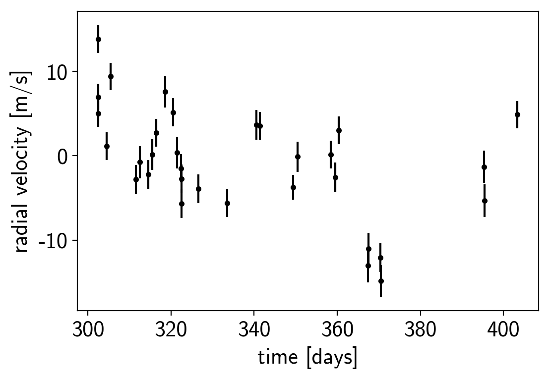
Then the RVs from RadVel:
import pandas as pd

url = "https://raw.githubusercontent.com/California-Planet-Search/radvel/master/example_data/epic203771098.csv"
data = pd.read_csv(url, index_col=0)

# Don't forget to remove the time offset from above!
x_rv = np.array(data.t) - x_ref
y_rv = np.array(data.vel)
yerr_rv = np.array(data.errvel)

plt.errorbar(x_rv, y_rv, yerr=yerr_rv, fmt=".k")
plt.xlabel("time [days]")
plt.ylabel("radial velocity [m/s]");
We can initialize the transit parameters using the box least squares periodogram from AstroPy. (Note: you’ll need AstroPy v3.1 or more recent to use this feature.) A full discussion of transit detection and vetting is beyond the scope of this tutorial so let’s assume that we know that there are two periodic transiting planets in this dataset.
from astropy.stats import BoxLeastSquares

m = np.zeros(len(x), dtype=bool)
period_grid = np.exp(np.linspace(np.log(5), np.log(50), 50000))
bls_results = []
periods = []
t0s = []
depths = []

# Compute the periodogram for each planet by iteratively masking out
# transits from the higher signal to noise planets. Here we're assuming
# that we know that there are exactly two planets.
for i in range(2):
    bls = BoxLeastSquares(x[~m], y[~m] - smooth[~m])
    bls_power = bls.power(period_grid, 0.1, oversample=20)
    bls_results.append(bls_power)

    # Save the highest peak as the planet candidate
    index = np.argmax(bls_power.power)
    periods.append(bls_power.period[index])
    t0s.append(bls_power.transit_time[index])
    depths.append(bls_power.depth[index])

    # Mask the data points that are in transit for this candidate
    m |= bls.transit_mask(x, periods[-1], 0.5, t0s[-1])
Let’s plot the initial transit estimates based on these periodograms:
fig, axes = plt.subplots(len(bls_results), 2, figsize=(15, 10))

for i in range(len(bls_results)):
    # Plot the periodogram
    ax = axes[i, 0]
    ax.axvline(np.log10(periods[i]), color="C1", lw=5, alpha=0.8)
    ax.plot(np.log10(bls_results[i].period), bls_results[i].power, "k")
    ax.annotate("period = {0:.4f} d".format(periods[i]),
                (0, 1), xycoords="axes fraction",
                xytext=(5, -5), textcoords="offset points",
                va="top", ha="left", fontsize=12)
    ax.set_ylabel("bls power")
    ax.set_yticks([])
    ax.set_xlim(np.log10(period_grid.min()), np.log10(period_grid.max()))
    if i < len(bls_results) - 1:
        ax.set_xticklabels([])
    else:
        ax.set_xlabel("log10(period)")

    # Plot the folded transit
    ax = axes[i, 1]
    p = periods[i]
    x_fold = (x - t0s[i] + 0.5*p) % p - 0.5*p
    m = np.abs(x_fold) < 0.4
    ax.plot(x_fold[m], y[m] - smooth[m], ".k")

    # Overplot the phase binned light curve
    bins = np.linspace(-0.41, 0.41, 32)
    denom, _ = np.histogram(x_fold, bins)
    num, _ = np.histogram(x_fold, bins, weights=y - smooth)
    denom[num == 0] = 1.0
    ax.plot(0.5*(bins[1:] + bins[:-1]), num / denom, color="C1")

    ax.set_xlim(-0.4, 0.4)
    ax.set_ylabel("relative flux [ppt]")
    if i < len(bls_results) - 1:
        ax.set_xticklabels([])
    else:
        ax.set_xlabel("time since transit")

fig.subplots_adjust(hspace=0.02)
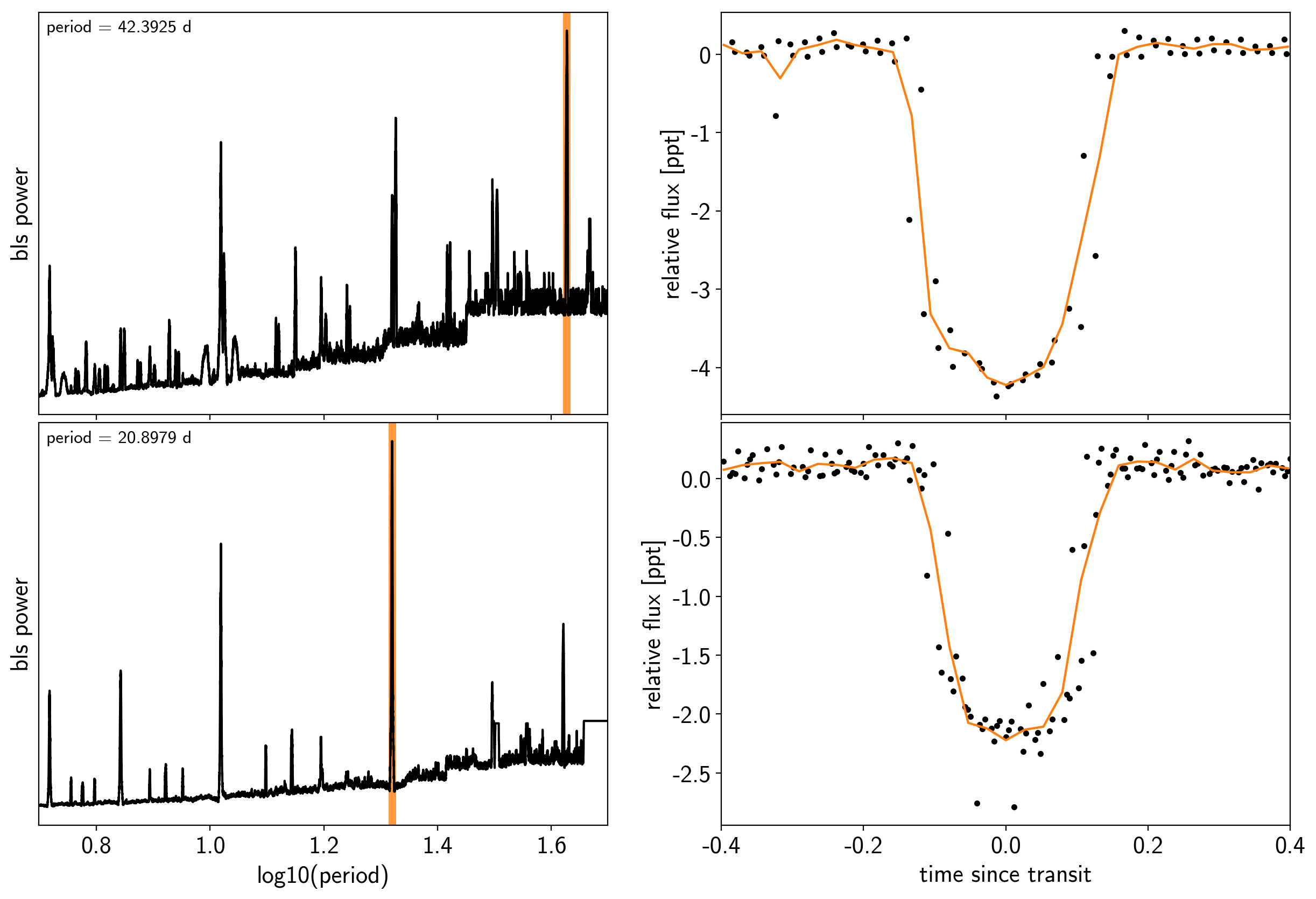
The discovery paper for K2-24 (Petigura et al. (2016)) includes the following estimates of the stellar mass and radius in Solar units:
M_star_petigura = 1.12, 0.05
R_star_petigura = 1.21, 0.11
Finally, using this stellar mass, we can also estimate the minimum masses of the planets given these transit parameters.
import exoplanet as xo
import astropy.units as u

msini = xo.estimate_minimum_mass(periods, x_rv, y_rv, yerr_rv, t0s=t0s, m_star=M_star_petigura[0])
msini = msini.to(u.M_earth)
print(msini)
[32.80060146 23.89885976] earthMass
A joint transit and radial velocity model in PyMC3
Now, let’s define our full model in PyMC3. There’s a lot going on here, but I’ve tried to comment it and most of it should be familiar from the previous tutorials (Radial velocity fitting, Transit fitting, Scalable Gaussian processes in PyMC3, and Gaussian process models for stellar variability). In this case, I’ve put the model inside a model “factory” function because we’ll do some sigma clipping below.
import pymc3 as pm
import theano.tensor as tt

t_rv = np.linspace(x_rv.min()-5, x_rv.max()+5, 1000)

def build_model(mask=None, start=None):
    if mask is None:
        mask = np.ones(len(x), dtype=bool)
    with pm.Model() as model:

        # Parameters for the stellar properties
        mean = pm.Normal("mean", mu=0.0, sd=10.0)
        u_star = xo.distributions.QuadLimbDark("u_star")
        BoundedNormal = pm.Bound(pm.Normal, lower=0, upper=3)
        m_star = BoundedNormal("m_star", mu=M_star_petigura[0], sd=M_star_petigura[1])
        r_star = BoundedNormal("r_star", mu=R_star_petigura[0], sd=R_star_petigura[1])

        # Orbital parameters for the planets
        logm = pm.Normal("logm", mu=np.log(msini.value), sd=1, shape=2)
        logP = pm.Normal("logP", mu=np.log(periods), sd=1, shape=2)
        t0 = pm.Normal("t0", mu=np.array(t0s), sd=1, shape=2)
        logr = pm.Normal("logr", mu=0.5*np.log(1e-3*np.array(depths)) + np.log(R_star_petigura[0]),
                         sd=1.0, shape=2)
        r_pl = pm.Deterministic("r_pl", tt.exp(logr))
        ror = pm.Deterministic("ror", r_pl / r_star)
        b = pm.Flat("b", shape=2,
                    transform=pm.distributions.transforms.logodds,
                    testval=0.5+np.zeros(2))

        # This is the eccentricity prior from Kipping (2013):
        # https://arxiv.org/abs/1306.4982
        BoundedBeta = pm.Bound(pm.Beta, lower=0, upper=1-1e-5)
        ecc = BoundedBeta("ecc", alpha=0.867, beta=3.03, shape=2,
                          testval=np.array([0.1, 0.1]))
        omega = xo.distributions.Angle("omega", shape=2)

        # RV jitter & a quadratic RV trend
        logs_rv = pm.Normal("logs_rv", mu=np.log(np.median(yerr_rv)), sd=5)
        trend = pm.Normal("trend", mu=0, sd=10.0**-np.arange(3)[::-1], shape=3)

        # Transit jitter & GP parameters
        logs2 = pm.Normal("logs2", mu=np.log(np.var(y[mask])), sd=10)
        logw0_guess = np.log(2*np.pi/10)
        logw0 = pm.Normal("logw0", mu=logw0_guess, sd=10)

        # We'll parameterize using the maximum power (S_0 * w_0^4) instead of
        # S_0 directly because this removes some of the degeneracies between
        # S_0 and omega_0
        logpower = pm.Normal("logpower",
                             mu=np.log(np.var(y[mask]))+4*logw0_guess,
                             sd=10)
        logS0 = pm.Deterministic("logS0", logpower - 4 * logw0)

        # Tracking planet parameters
        period = pm.Deterministic("period", tt.exp(logP))
        m_pl = pm.Deterministic("m_pl", tt.exp(logm))

        # Orbit model
        orbit = xo.orbits.KeplerianOrbit(
            r_star=r_star, m_star=m_star,
            period=period, t0=t0, b=b, m_planet=m_pl,
            ecc=ecc, omega=omega,
            m_planet_units=msini.unit)

        # Compute the model light curve using starry
        light_curves = xo.StarryLightCurve(u_star).get_light_curve(
            orbit=orbit, r=r_pl, t=x[mask], texp=texp)*1e3
        light_curve = pm.math.sum(light_curves, axis=-1) + mean
        pm.Deterministic("light_curves", light_curves)

        # GP model for the light curve
        kernel = xo.gp.terms.SHOTerm(log_S0=logS0, log_w0=logw0, Q=1/np.sqrt(2))
        gp = xo.gp.GP(kernel, x[mask], tt.exp(logs2) + tt.zeros(mask.sum()), J=2)
        pm.Potential("transit_obs", gp.log_likelihood(y[mask] - light_curve))
        pm.Deterministic("gp_pred", gp.predict())

        # Set up the RV model and save it as a deterministic
        # for plotting purposes later
        vrad = orbit.get_radial_velocity(x_rv)
        pm.Deterministic("vrad", vrad)

        # Define the background RV model
        A = np.vander(x_rv - 0.5*(x_rv.min() + x_rv.max()), 3)
        bkg = pm.Deterministic("bkg", tt.dot(A, trend))

        # The likelihood for the RVs
        rv_model = pm.Deterministic("rv_model", tt.sum(vrad, axis=-1) + bkg)
        err = tt.sqrt(yerr_rv**2 + tt.exp(2*logs_rv))
        pm.Normal("obs", mu=rv_model, sd=err, observed=y_rv)

        vrad_pred = orbit.get_radial_velocity(t_rv)
        pm.Deterministic("vrad_pred", vrad_pred)
        A_pred = np.vander(t_rv - 0.5*(x_rv.min() + x_rv.max()), 3)
        bkg_pred = pm.Deterministic("bkg_pred", tt.dot(A_pred, trend))
        pm.Deterministic("rv_model_pred", tt.sum(vrad_pred, axis=-1) + bkg_pred)

        # Fit for the maximum a posteriori parameters, I've found that I can get
        # a better solution by trying different combinations of parameters in turn
        if start is None:
            start = model.test_point
        map_soln = xo.optimize(start=start, vars=[trend])
        map_soln = xo.optimize(start=map_soln, vars=[logs2])
        map_soln = xo.optimize(start=map_soln, vars=[logr, b])
        map_soln = xo.optimize(start=map_soln, vars=[logP, t0])
        map_soln = xo.optimize(start=map_soln, vars=[logs2, logpower])
        map_soln = xo.optimize(start=map_soln, vars=[logw0])
        map_soln = xo.optimize(start=map_soln)
        map_soln = xo.optimize(start=map_soln, vars=[logm, ecc, omega])
        map_soln = xo.optimize(start=map_soln)

    return model, map_soln
model0, map_soln0 = build_model()
optimizing logp for variables: ['trend']
message: Optimization terminated successfully.
logp: -8250.572319847692 -> -8233.972126547622
optimizing logp for variables: ['logs2']
message: Optimization terminated successfully.
logp: -8233.972126547622 -> 1985.195383239683
optimizing logp for variables: ['b_logodds__', 'logr']
message: Desired error not necessarily achieved due to precision loss.
logp: 1985.195383239683 -> 2679.698211591958
optimizing logp for variables: ['t0', 'logP']
message: Desired error not necessarily achieved due to precision loss.
logp: 2679.698211591958 -> 3334.2117904820097
optimizing logp for variables: ['logpower', 'logs2']
message: Optimization terminated successfully.
logp: 3334.2117904820097 -> 4291.602174987188
optimizing logp for variables: ['logw0']
message: Optimization terminated successfully.
logp: 4291.602174987188 -> 4365.5542833298605
optimizing logp for variables: ['logpower', 'logw0', 'logs2', 'trend', 'logs_rv', 'omega_angle__', 'ecc_interval__', 'b_logodds__', 'logr', 't0', 'logP', 'logm', 'r_star_interval__', 'm_star_interval__', 'u_star_quadlimbdark__', 'mean']
message: Desired error not necessarily achieved due to precision loss.
logp: 4365.5542833298605 -> 4777.103510779301
optimizing logp for variables: ['omega_angle__', 'ecc_interval__', 'logm']
message: Desired error not necessarily achieved due to precision loss.
logp: 4777.103510779301 -> 4777.103510779483
optimizing logp for variables: ['logpower', 'logw0', 'logs2', 'trend', 'logs_rv', 'omega_angle__', 'ecc_interval__', 'b_logodds__', 'logr', 't0', 'logP', 'logm', 'r_star_interval__', 'm_star_interval__', 'u_star_quadlimbdark__', 'mean']
message: Desired error not necessarily achieved due to precision loss.
logp: 4777.103510779483 -> 4777.103510779483
Now let’s plot the map radial velocity model.
def plot_rv_curve(soln):
    fig, axes = plt.subplots(2, 1, figsize=(10, 5), sharex=True)

    ax = axes[0]
    ax.errorbar(x_rv, y_rv, yerr=yerr_rv, fmt=".k")
    ax.plot(t_rv, soln["vrad_pred"], "--k", alpha=0.5)
    ax.plot(t_rv, soln["bkg_pred"], ":k", alpha=0.5)
    ax.plot(t_rv, soln["rv_model_pred"], label="model")
    ax.legend(fontsize=10)
    ax.set_ylabel("radial velocity [m/s]")

    ax = axes[1]
    err = np.sqrt(yerr_rv**2+np.exp(2*soln["logs_rv"]))
    ax.errorbar(x_rv, y_rv - soln["rv_model"], yerr=err, fmt=".k")
    ax.axhline(0, color="k", lw=1)
    ax.set_ylabel("residuals [m/s]")
    ax.set_xlim(t_rv.min(), t_rv.max())
    ax.set_xlabel("time [days]")

plot_rv_curve(map_soln0)
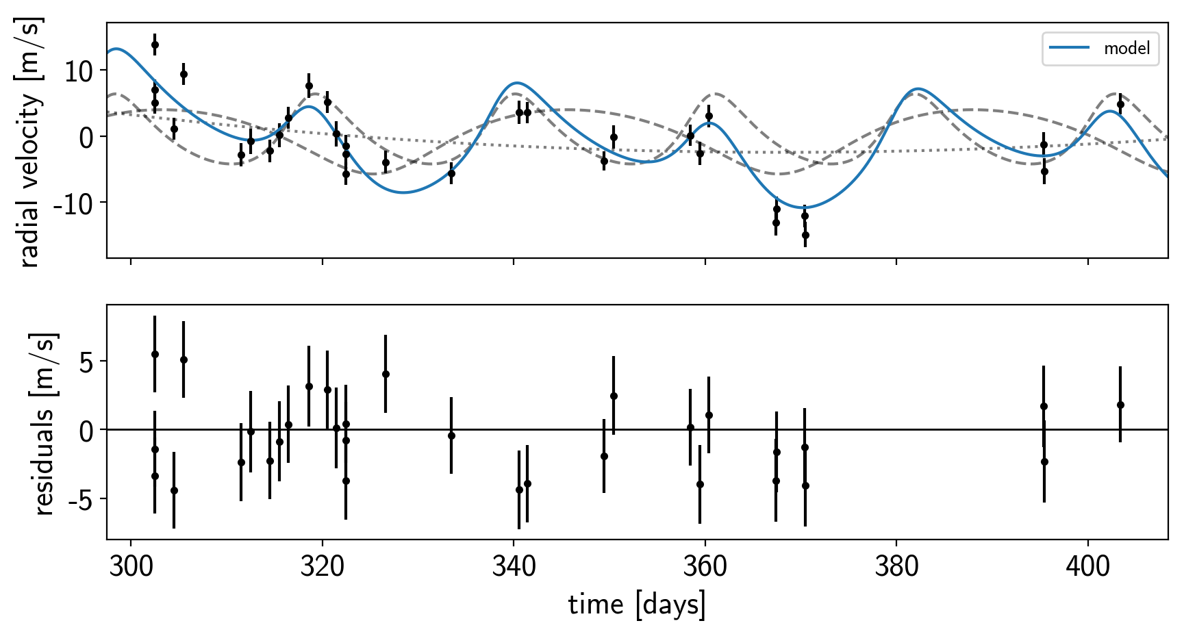
That looks pretty similar to what we got in Radial velocity fitting. Now let’s also plot the transit model.
def plot_light_curve(soln, mask=None):
    if mask is None:
        mask = np.ones(len(x), dtype=bool)

    fig, axes = plt.subplots(3, 1, figsize=(10, 7), sharex=True)

    ax = axes[0]
    ax.plot(x[mask], y[mask], "k", label="data")
    gp_mod = soln["gp_pred"] + soln["mean"]
    ax.plot(x[mask], gp_mod, color="C2", label="gp model")
    ax.legend(fontsize=10)
    ax.set_ylabel("relative flux [ppt]")

    ax = axes[1]
    ax.plot(x[mask], y[mask] - gp_mod, "k", label="de-trended data")
    for i, l in enumerate("bc"):
        mod = soln["light_curves"][:, i]
        ax.plot(x[mask], mod, label="planet {0}".format(l))
    ax.legend(fontsize=10, loc=3)
    ax.set_ylabel("de-trended flux [ppt]")

    ax = axes[2]
    mod = gp_mod + np.sum(soln["light_curves"], axis=-1)
    ax.plot(x[mask], y[mask] - mod, "k")
    ax.axhline(0, color="#aaaaaa", lw=1)
    ax.set_ylabel("residuals [ppt]")
    ax.set_xlim(x[mask].min(), x[mask].max())
    ax.set_xlabel("time [days]")

    return fig

plot_light_curve(map_soln0);
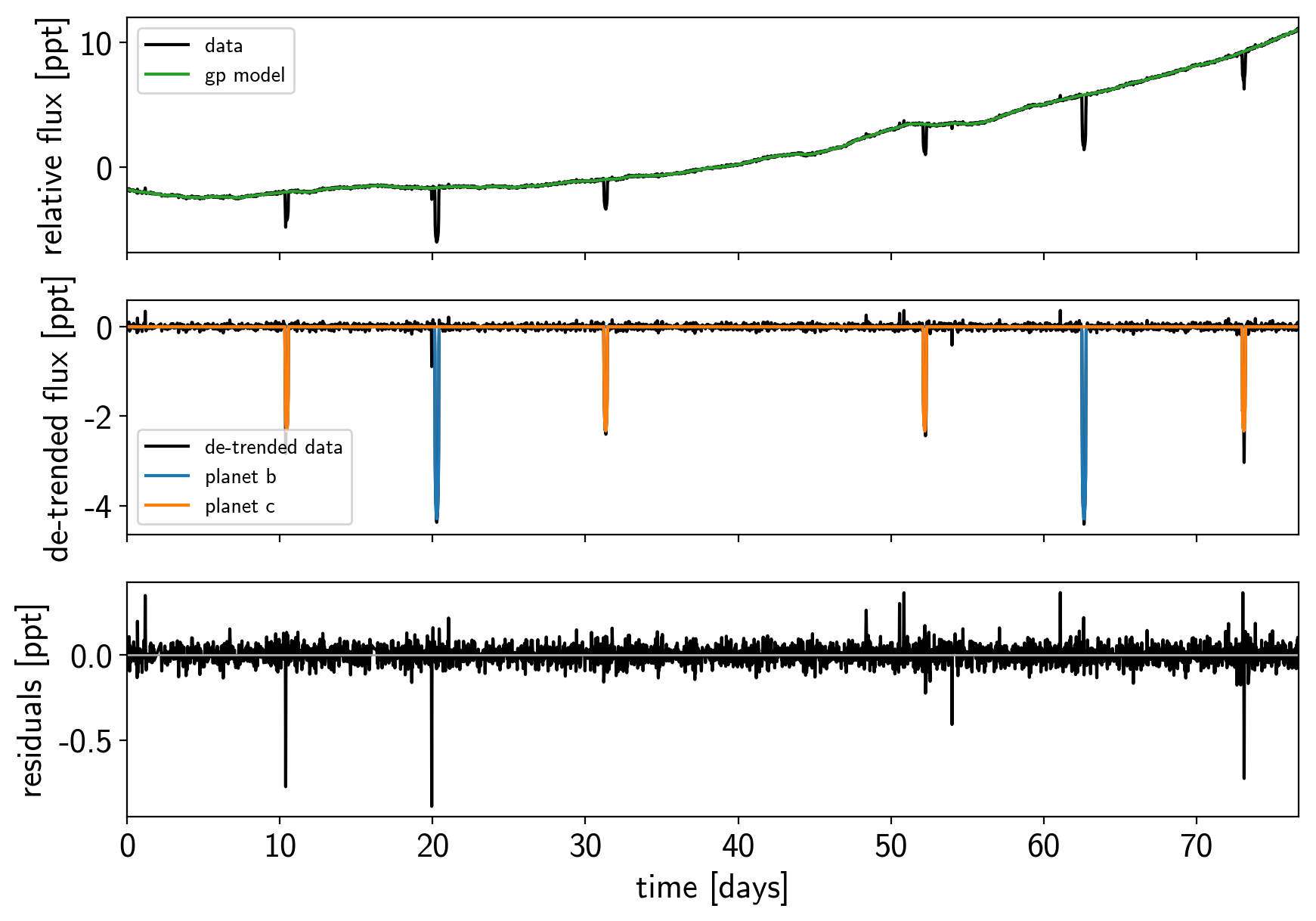
There are still a few outliers in the light curve and it can be useful to remove those before doing the full fit because both the GP and transit parameters can be sensitive to this.
Sigma clipping
To remove the outliers, we’ll look at the empirical RMS of the residuals away from the GP + transit model and remove anything that is more than a 7-sigma outlier.
mod = map_soln0["gp_pred"] + map_soln0["mean"] + np.sum(map_soln0["light_curves"], axis=-1)
resid = y - mod
rms = np.sqrt(np.median(resid**2))
mask = np.abs(resid) < 7 * rms

plt.plot(x, resid, "k", label="data")
plt.plot(x[~mask], resid[~mask], "xr", label="outliers")
plt.axhline(0, color="#aaaaaa", lw=1)
plt.ylabel("residuals [ppt]")
plt.xlabel("time [days]")
plt.legend(fontsize=12, loc=4)
plt.xlim(x.min(), x.max());
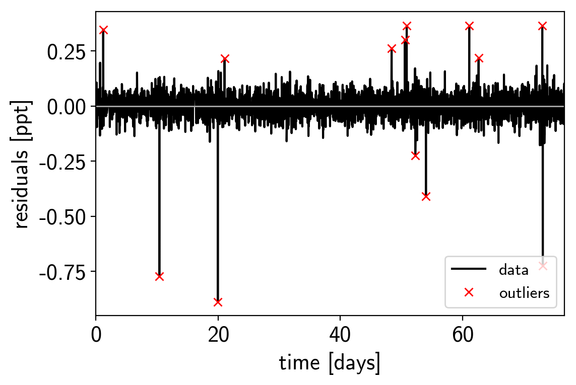
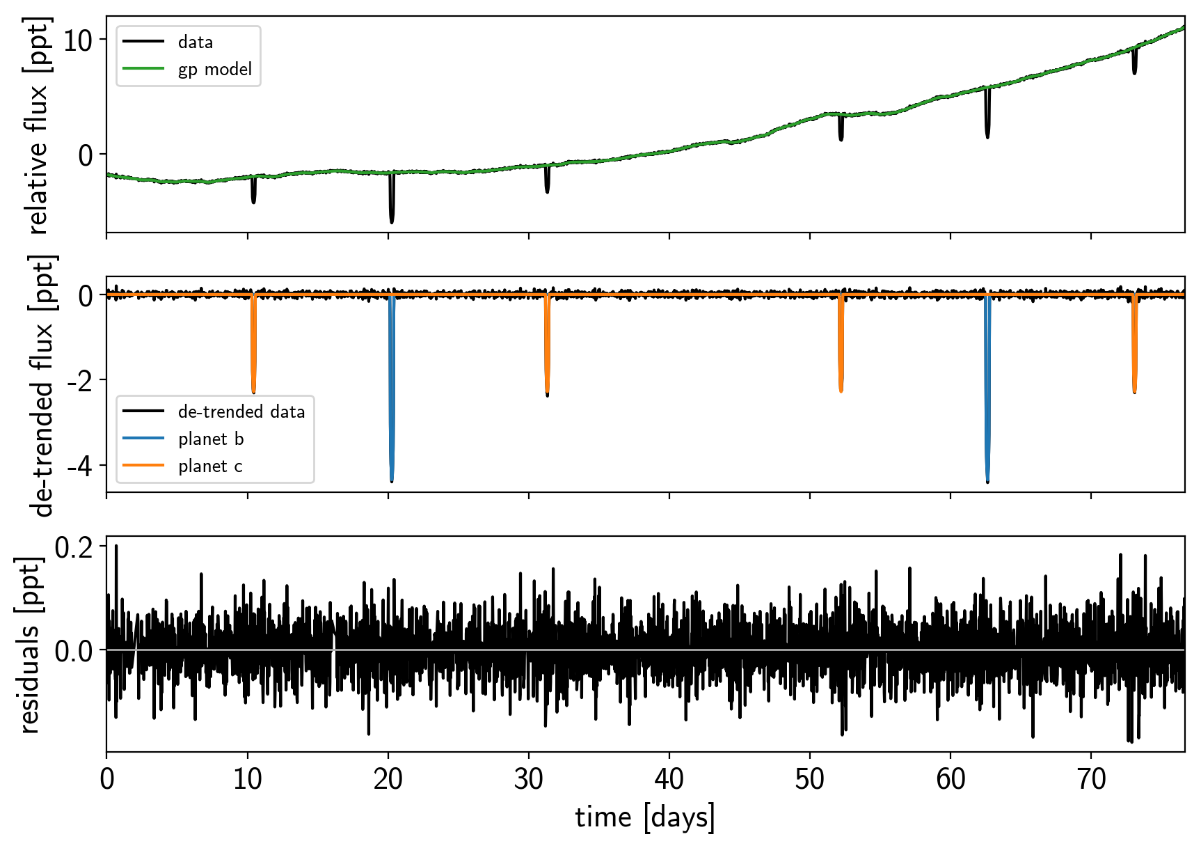
That looks better. Let’s re-build our model with this sigma-clipped dataset.
model, map_soln = build_model(mask, map_soln0)
plot_light_curve(map_soln, mask);
optimizing logp for variables: ['trend']
message: Optimization terminated successfully.
logp: 5227.116869460895 -> 5227.116869460898
optimizing logp for variables: ['logs2']
message: Desired error not necessarily achieved due to precision loss.
logp: 5227.116869460898 -> 5309.2239182160365
optimizing logp for variables: ['b_logodds__', 'logr']
message: Desired error not necessarily achieved due to precision loss.
logp: 5309.223918216018 -> 5320.261376226418
optimizing logp for variables: ['t0', 'logP']
message: Desired error not necessarily achieved due to precision loss.
logp: 5320.261376226418 -> 5321.717901372164
optimizing logp for variables: ['logpower', 'logs2']
message: Optimization terminated successfully.
logp: 5321.717901372168 -> 5322.452093012708
optimizing logp for variables: ['logw0']
message: Optimization terminated successfully.
logp: 5322.452093012708 -> 5322.486343182219
optimizing logp for variables: ['logpower', 'logw0', 'logs2', 'trend', 'logs_rv', 'omega_angle__', 'ecc_interval__', 'b_logodds__', 'logr', 't0', 'logP', 'logm', 'r_star_interval__', 'm_star_interval__', 'u_star_quadlimbdark__', 'mean']
message: Desired error not necessarily achieved due to precision loss.
logp: 5322.486343182217 -> 5324.3056735786095
optimizing logp for variables: ['omega_angle__', 'ecc_interval__', 'logm']
message: Desired error not necessarily achieved due to precision loss.
logp: 5324.3056735786095 -> 5324.3056735786095
optimizing logp for variables: ['logpower', 'logw0', 'logs2', 'trend', 'logs_rv', 'omega_angle__', 'ecc_interval__', 'b_logodds__', 'logr', 't0', 'logP', 'logm', 'r_star_interval__', 'm_star_interval__', 'u_star_quadlimbdark__', 'mean']
message: Desired error not necessarily achieved due to precision loss.
logp: 5324.3056735786095 -> 5324.3056735786095
Great! Now we’re ready to sample.
Sampling
The sampling for this model is the same as for all the previous tutorials, but it takes a bit longer (about 2 hours on my laptop). This is partly because the model is more expensive to compute than the previous ones and partly because there are some non-affine degeneracies in the problem (for example between impact parameter and eccentricity). It might be worth thinking about reparameterizations (in terms of duration instead of eccentricity), but that’s beyond the scope of this tutorial. Besides, using more traditional MCMC methods, this would have taken a lot more than 2 hours to get >1000 effective samples!
np.random.seed(123)
sampler = xo.PyMC3Sampler(finish=500, chains=4)
with model:
    burnin = sampler.tune(tune=4500, start=map_soln,
                          step_kwargs=dict(target_accept=0.95))
Sampling 4 chains: 100%|██████████| 308/308 [00:50<00:00,  1.98draws/s]
Sampling 4 chains: 100%|██████████| 108/108 [00:17<00:00,  1.46draws/s]
Sampling 4 chains: 100%|██████████| 208/208 [00:38<00:00,  1.95draws/s]
Sampling 4 chains: 100%|██████████| 408/408 [01:06<00:00,  1.33draws/s]
Sampling 4 chains: 100%|██████████| 808/808 [02:12<00:00,  2.12draws/s]
Sampling 4 chains: 100%|██████████| 1608/1608 [05:48<00:00,  1.27draws/s]
Sampling 4 chains: 100%|██████████| 3208/3208 [10:14<00:00,  1.65draws/s]
Sampling 4 chains: 100%|██████████| 11408/11408 [36:30<00:00,  1.50draws/s]
Sampling 4 chains: 100%|██████████| 2008/2008 [06:23<00:00,  5.23draws/s]
with model:
    trace = sampler.sample(draws=3000)
Multiprocess sampling (4 chains in 4 jobs)
NUTS: [logpower, logw0, logs2, trend, logs_rv, omega, ecc, b, logr, t0, logP, logm, r_star, m_star, u_star, mean]
Sampling 4 chains: 100%|██████████| 12000/12000 [36:15<00:00,  1.32draws/s]
There were 28 divergences after tuning. Increase target_accept or reparameterize.
There were 15 divergences after tuning. Increase target_accept or reparameterize.
There were 21 divergences after tuning. Increase target_accept or reparameterize.
There were 30 divergences after tuning. Increase target_accept or reparameterize.
The number of effective samples is smaller than 10% for some parameters.
Let’s look at the convergence diagnostics for some of the key parameters:
pm.summary(trace, varnames=["period", "r_pl", "m_pl", "ecc", "omega", "b"])
| mean | sd | mc_error | hpd_2.5 | hpd_97.5 | n_eff | Rhat | |
|---|---|---|---|---|---|---|---|
| period__0 | 42.363460 | 0.000405 | 0.000003 | 42.362691 | 42.364285 | 13474.651185 | 1.000101 |
| period__1 | 20.885346 | 0.000204 | 0.000002 | 20.884950 | 20.885749 | 12713.048399 | 0.999959 |
| r_pl__0 | 0.077569 | 0.004944 | 0.000083 | 0.067145 | 0.086772 | 2715.855335 | 1.001357 |
| r_pl__1 | 0.056501 | 0.003859 | 0.000070 | 0.048498 | 0.063825 | 2326.592772 | 1.001489 |
| m_pl__0 | 28.242430 | 5.600593 | 0.050261 | 17.218559 | 39.156167 | 10218.499949 | 1.000031 |
| m_pl__1 | 23.048895 | 4.065473 | 0.042467 | 14.670690 | 30.803872 | 9044.495916 | 1.000054 |
| ecc__0 | 0.085489 | 0.074193 | 0.001295 | 0.000005 | 0.238402 | 2682.994846 | 1.000826 |
| ecc__1 | 0.203971 | 0.078988 | 0.001514 | 0.034378 | 0.348774 | 2416.227878 | 1.000272 |
| omega__0 | -0.055880 | 2.269985 | 0.035895 | -3.137120 | 3.021119 | 3440.612885 | 1.000640 |
| omega__1 | -0.484615 | 0.493323 | 0.012935 | -1.351781 | 0.529525 | 1608.914593 | 1.003896 |
| b__0 | 0.589653 | 0.046685 | 0.000814 | 0.498551 | 0.670171 | 3109.427786 | 1.001295 |
| b__1 | 0.587727 | 0.107282 | 0.003126 | 0.356377 | 0.740683 | 1199.357292 | 1.002787 |
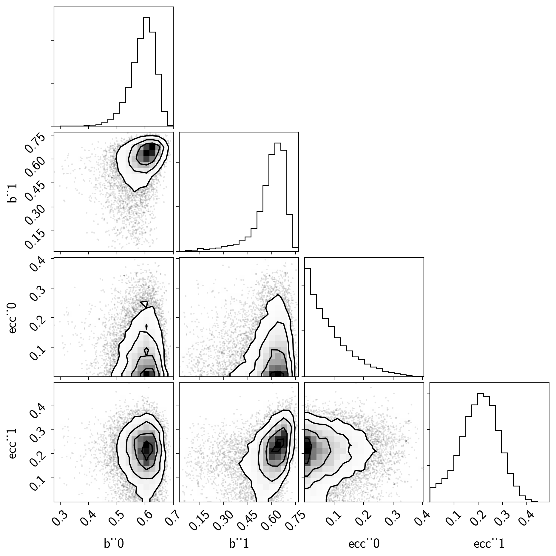
As you see, the effective number of samples for the impact parameters and eccentricites are lower than for the other parameters. This is because of the correlations that I mentioned above:
import corner
varnames = ["b", "ecc"]
samples = pm.trace_to_dataframe(trace, varnames=varnames)
fig = corner.corner(samples);
Phase plots
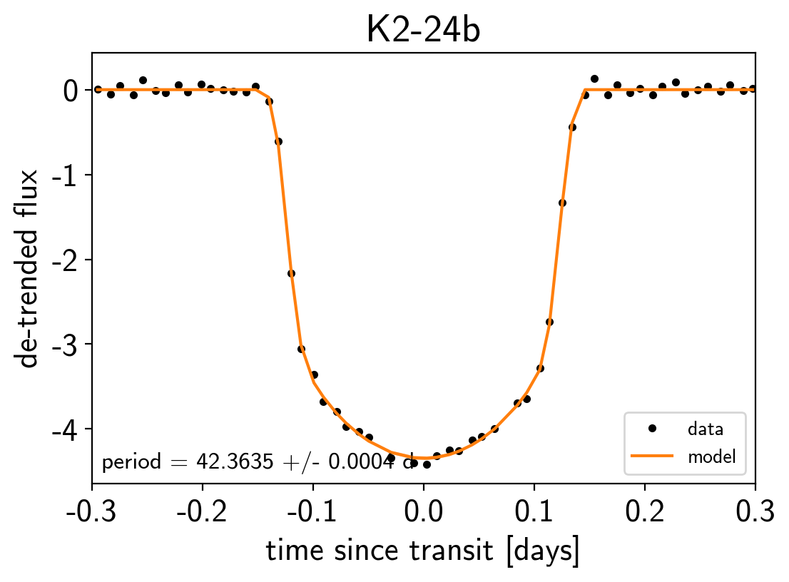
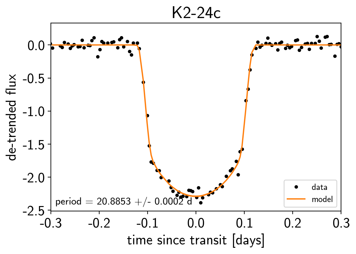
Finally, as in the Radial velocity fitting and Transit fitting tutorials, we can make folded plots of the transits and the radial velocities and compare to the posterior model predictions. (Note: planets b and c in this tutorial are swapped compared to the labels from Petigura et al. (2016))
for n, letter in enumerate("bc"):
    plt.figure()

    # Compute the GP prediction
    gp_mod = np.median(trace["gp_pred"] + trace["mean"][:, None], axis=0)

    # Get the posterior median orbital parameters
    p = np.median(trace["period"][:, n])
    t0 = np.median(trace["t0"][:, n])

    # Compute the median of posterior estimate of the contribution from
    # the other planet. Then we can remove this from the data to plot
    # just the planet we care about.
    other = np.median(trace["light_curves"][:, :, (n + 1) % 2], axis=0)

    # Plot the folded data
    x_fold = (x[mask] - t0 + 0.5*p) % p - 0.5*p
    plt.plot(x_fold, y[mask] - gp_mod - other, ".k", label="data", zorder=-1000)

    # Plot the folded model
    inds = np.argsort(x_fold)
    inds = inds[np.abs(x_fold)[inds] < 0.3]
    pred = trace["light_curves"][:, inds, n]
    pred = np.percentile(pred, [16, 50, 84], axis=0)
    plt.plot(x_fold[inds], pred[1], color="C1", label="model")
    art = plt.fill_between(x_fold[inds], pred[0], pred[2], color="C1", alpha=0.5,
                           zorder=1000)
    art.set_edgecolor("none")

    # Annotate the plot with the planet's period
    txt = "period = {0:.4f} +/- {1:.4f} d".format(
        np.mean(trace["period"][:, n]), np.std(trace["period"][:, n]))
    plt.annotate(txt, (0, 0), xycoords="axes fraction",
                 xytext=(5, 5), textcoords="offset points",
                 ha="left", va="bottom", fontsize=12)

    plt.legend(fontsize=10, loc=4)
    plt.xlim(-0.5*p, 0.5*p)
    plt.xlabel("time since transit [days]")
    plt.ylabel("de-trended flux")
    plt.title("K2-24{0}".format(letter));
    plt.xlim(-0.3, 0.3)
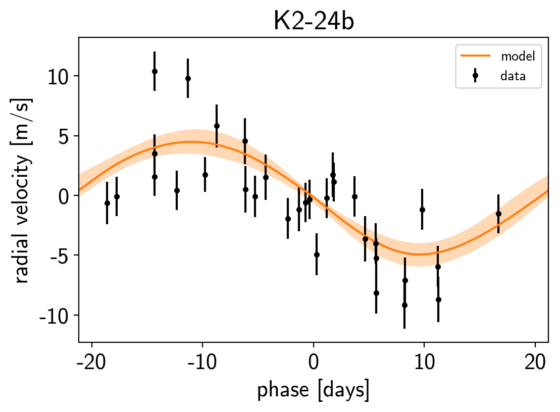
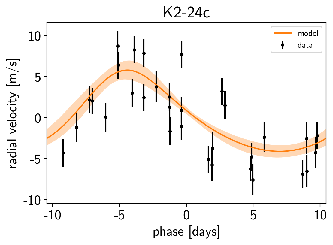
for n, letter in enumerate("bc"):
    plt.figure()

    # Get the posterior median orbital parameters
    p = np.median(trace["period"][:, n])
    t0 = np.median(trace["t0"][:, n])

    # Compute the median of posterior estimate of the background RV
    # and the contribution from the other planet. Then we can remove
    # this from the data to plot just the planet we care about.
    other = np.median(trace["vrad"][:, :, (n + 1) % 2], axis=0)
    other += np.median(trace["bkg"], axis=0)

    # Plot the folded data
    x_fold = (x_rv - t0 + 0.5*p) % p - 0.5*p
    plt.errorbar(x_fold, y_rv - other, yerr=yerr_rv, fmt=".k", label="data")

    # Compute the posterior prediction for the folded RV model for this
    # planet
    t_fold = (t_rv - t0 + 0.5*p) % p - 0.5*p
    inds = np.argsort(t_fold)
    pred = np.percentile(trace["vrad_pred"][:, inds, n], [16, 50, 84], axis=0)
    plt.plot(t_fold[inds], pred[1], color="C1", label="model")
    art = plt.fill_between(t_fold[inds], pred[0], pred[2], color="C1", alpha=0.3)
    art.set_edgecolor("none")

    plt.legend(fontsize=10)
    plt.xlim(-0.5*p, 0.5*p)
    plt.xlabel("phase [days]")
    plt.ylabel("radial velocity [m/s]")
    plt.title("K2-24{0}".format(letter));
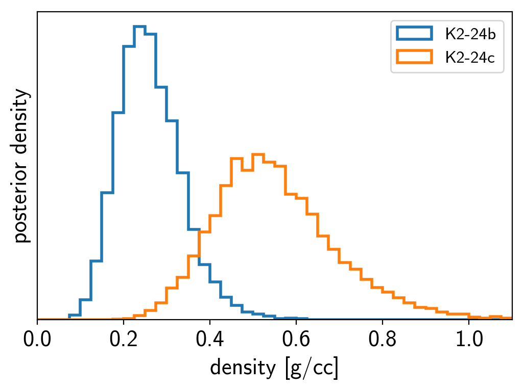
We can also compute the posterior constraints on the planet densities.
volume = 4/3*np.pi*trace["r_pl"]**3
density = u.Quantity(trace["m_pl"] / volume, unit=u.M_earth / u.R_sun**3)
density = density.to(u.g / u.cm**3).value

bins = np.linspace(0, 1.1, 45)
for n, letter in enumerate("bc"):
    plt.hist(density[:, n], bins, histtype="step", lw=2,
             label="K2-24{0}".format(letter), density=True)
plt.yticks([])
plt.legend(fontsize=12)
plt.xlim(bins[0], bins[-1])
plt.xlabel("density [g/cc]")
plt.ylabel("posterior density");
Citations
As described in the Citing exoplanet & its dependencies tutorial, we can use
exoplanet.citations.get_citations_for_model() to construct an
acknowledgement and BibTeX listing that includes the relevant citations
for this model.
with model:
    txt, bib = xo.citations.get_citations_for_model()
print(txt)
This research made use of textsf{exoplanet} citep{exoplanet} and its
dependencies citep{exoplanet:astropy13, exoplanet:astropy18,
exoplanet:exoplanet, exoplanet:foremanmackey17, exoplanet:foremanmackey18,
exoplanet:kipping13, exoplanet:luger18, exoplanet:pymc3, exoplanet:theano}.
print("\n".join(bib.splitlines()[:10]) + "\n...")
@misc{exoplanet:exoplanet,
  author = {Dan Foreman-Mackey and
            Geert Barentsen and
            Tom Barclay},
   title = {dfm/exoplanet: exoplanet v0.1.5},
   month = mar,
    year = 2019,
     doi = {10.5281/zenodo.2587222},
     url = {https://doi.org/10.5281/zenodo.2587222}
...