Note
This tutorial was generated from an IPython notebook that can be downloaded here.
theano version: 1.0.4
pymc3 version: 3.7
exoplanet version: 0.2.0
exoplanet comes bundled with a few utilities that can make it easier to use and debug PyMC3 models for fitting exoplanet data. This tutorial briefly describes these features and their use.
The main extra is the exoplanet.PyMC3Sampler class that wraps
the PyMC3 sampling procedure to include support for learning
off-diagonal elements of the mass matrix. This is very important for
any problems where there are covariances between the parameters (this is
true for pretty much all exoplanet models). A thorough discussion of
this can be found elsewhere
online, but here is a
simple demo where we sample a covariant Gaussian using
exoplanet.PyMC3Sampler.
First, we generate a random positive definite covariance matrix for the Gaussian:
import numpy as np

ndim = 5
np.random.seed(42)
L = np.random.randn(ndim, ndim)
L[np.diag_indices_from(L)] = 0.1*np.exp(L[np.diag_indices_from(L)])
L[np.triu_indices_from(L, 1)] = 0.0
cov = np.dot(L, L.T)
And then we can sample this using PyMC3 and
exoplanet.PyMC3Sampler:
import pymc3 as pm
import exoplanet as xo

sampler = xo.PyMC3Sampler()

with pm.Model() as model:
    pm.MvNormal("x", mu=np.zeros(ndim), chol=L, shape=(ndim,))

    # Run the burn-in and learn the mass matrix
    step_kwargs = dict(target_accept=0.9)
    sampler.tune(tune=2000, step_kwargs=step_kwargs, chains=4)

    # Run the production chain
    trace = sampler.sample(draws=2000, chains=4)
Sampling 4 chains: 100%|██████████| 308/308 [00:02<00:00, 123.14draws/s]
Sampling 4 chains: 100%|██████████| 108/108 [00:00<00:00, 133.09draws/s]
Sampling 4 chains: 100%|██████████| 208/208 [00:00<00:00, 759.13draws/s]
Sampling 4 chains: 100%|██████████| 408/408 [00:00<00:00, 1918.73draws/s]
Sampling 4 chains: 100%|██████████| 808/808 [00:00<00:00, 2551.37draws/s]
Sampling 4 chains: 100%|██████████| 1608/1608 [00:00<00:00, 2423.93draws/s]
Sampling 4 chains: 100%|██████████| 4608/4608 [00:01<00:00, 2559.72draws/s]
Sampling 4 chains: 100%|██████████| 208/208 [00:00<00:00, 1701.01draws/s]
Multiprocess sampling (4 chains in 4 jobs)
NUTS: [x]
Sampling 4 chains: 100%|██████████| 8000/8000 [00:02<00:00, 2840.62draws/s]
This is a little more verbose than the standard use of PyMC3, but the
performance is several orders of magnitude better than you would get
without the mass matrix tuning. As you can see from the
pymc3.summary, the autocorrelation time of this chain is about 1 as
we would expect for a simple problem like this.
pm.summary(trace)
| mean | sd | mc_error | hpd_2.5 | hpd_97.5 | n_eff | Rhat | |
|---|---|---|---|---|---|---|---|
| x__0 | 0.001067 | 0.168109 | 0.001667 | -0.336342 | 0.332161 | 10736.036303 | 1.000023 |
| x__1 | -0.007744 | 0.530522 | 0.005321 | -1.025180 | 1.028143 | 11458.853735 | 0.999766 |
| x__2 | 0.002726 | 0.678935 | 0.006146 | -1.343355 | 1.358254 | 11937.872184 | 1.000005 |
| x__3 | 0.008195 | 1.205641 | 0.010899 | -2.307936 | 2.460391 | 12428.450698 | 0.999940 |
| x__4 | 0.032899 | 2.091726 | 0.019298 | -4.369928 | 3.875477 | 10806.049803 | 1.000038 |
I find that when I’m debugging a PyMC3 model, I often want to inspect
the value of some part of the model for a given set of parameters. As
far as I can tell, there isn’t a simple way to do this in PyMC3, so
exoplanet comes with a hack for doing this:
exoplanet.eval_in_model(). This function handles the mapping
between named PyMC3 variables and the input required by the Theano
function that can evaluate the requested variable or tensor.
As a demo, let’s say that we’re fitting a parabola to some data:
np.random.seed(42)
x = np.sort(np.random.uniform(-1, 1, 50))
with pm.Model() as model:
    logs = pm.Normal("logs", mu=-3.0, sd=1.0)
    a0 = pm.Normal("a0")
    a1 = pm.Normal("a1")
    a2 = pm.Normal("a2")
    mod = a0 + a1 * x + a2 * x**2

    # Sample from the prior
    prior_sample = pm.sample_prior_predictive(samples=1)
    y = xo.eval_in_model(mod, prior_sample)
    y += np.exp(prior_sample["logs"]) * np.random.randn(len(y))

    # Add the likelihood
    pm.Normal("obs", mu=mod, sd=pm.math.exp(logs), observed=y)

    # Fit the data
    map_soln = xo.optimize()
    trace = pm.sample()
Auto-assigning NUTS sampler...
Initializing NUTS using jitter+adapt_diag...
optimizing logp for variables: ['a2', 'a1', 'a0', 'logs']
message: Optimization terminated successfully.
logp: -180.51036900636572 -> 42.72311721910288
Multiprocess sampling (4 chains in 4 jobs)
NUTS: [a2, a1, a0, logs]
Sampling 4 chains: 100%|██████████| 4000/4000 [00:01<00:00, 3186.09draws/s]
The acceptance probability does not match the target. It is 0.8788002200800235, but should be close to 0.8. Try to increase the number of tuning steps.
The acceptance probability does not match the target. It is 0.8834353310005734, but should be close to 0.8. Try to increase the number of tuning steps.
The acceptance probability does not match the target. It is 0.8827839735098203, but should be close to 0.8. Try to increase the number of tuning steps.
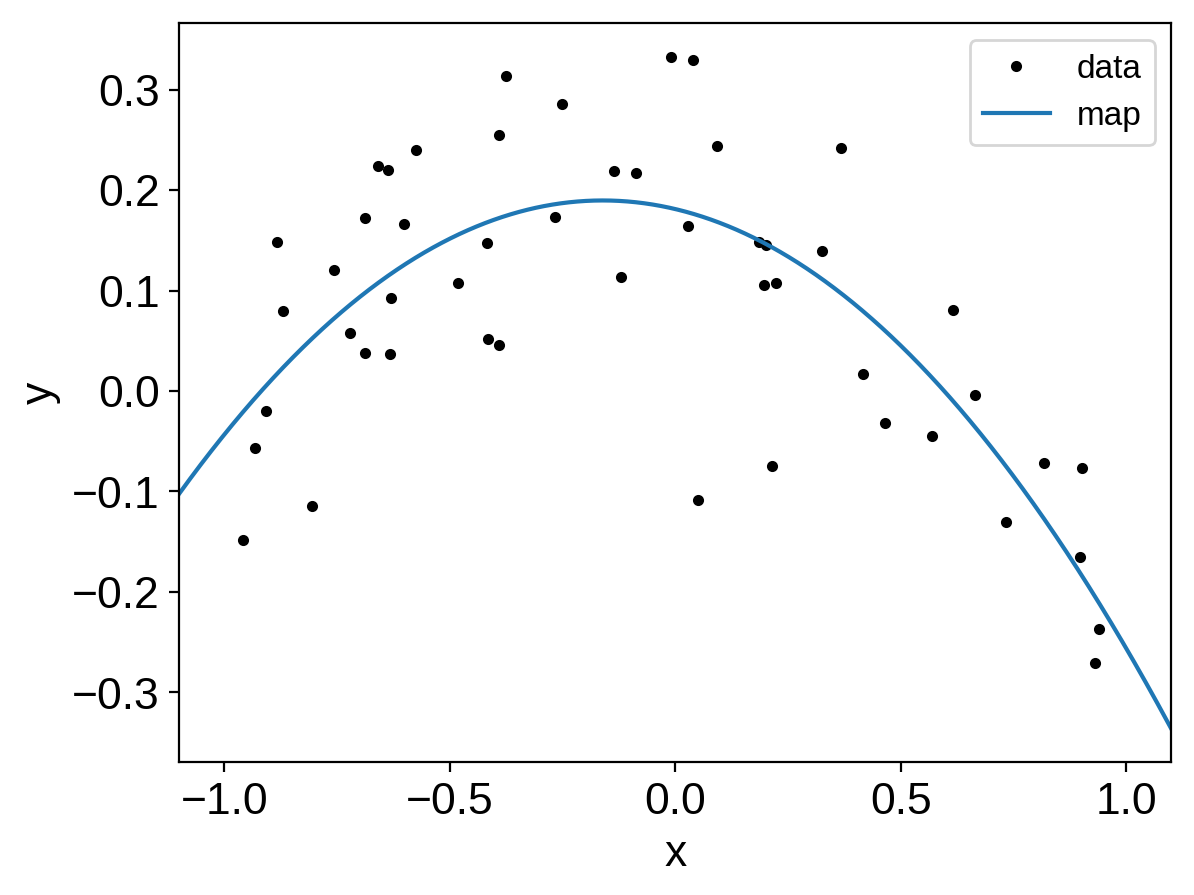
After running the fit, it might be interesting to look at the
predictions of the model. We could have added a pymc3.Deterministic
node for eveything, but that can end up taking up a lot of memory and
sometimes its useful to be able to experiement with different outputs.
Using exoplanet.utils.eval_in_model() we can, for example,
evaluate the maximum a posteriori (MAP) model prediction on a fine grid:
import matplotlib.pyplot as plt

x_grid = np.linspace(-1.1, 1.1, 5000)
with model:
    pred = xo.eval_in_model(a0 + a1 * x_grid + a2 * x_grid**2, map_soln)

plt.plot(x, y, ".k", label="data")
plt.plot(x_grid, pred, label="map")
plt.legend(fontsize=12)
plt.xlabel("x")
plt.ylabel("y")
plt.xlim(-1.1, 1.1);
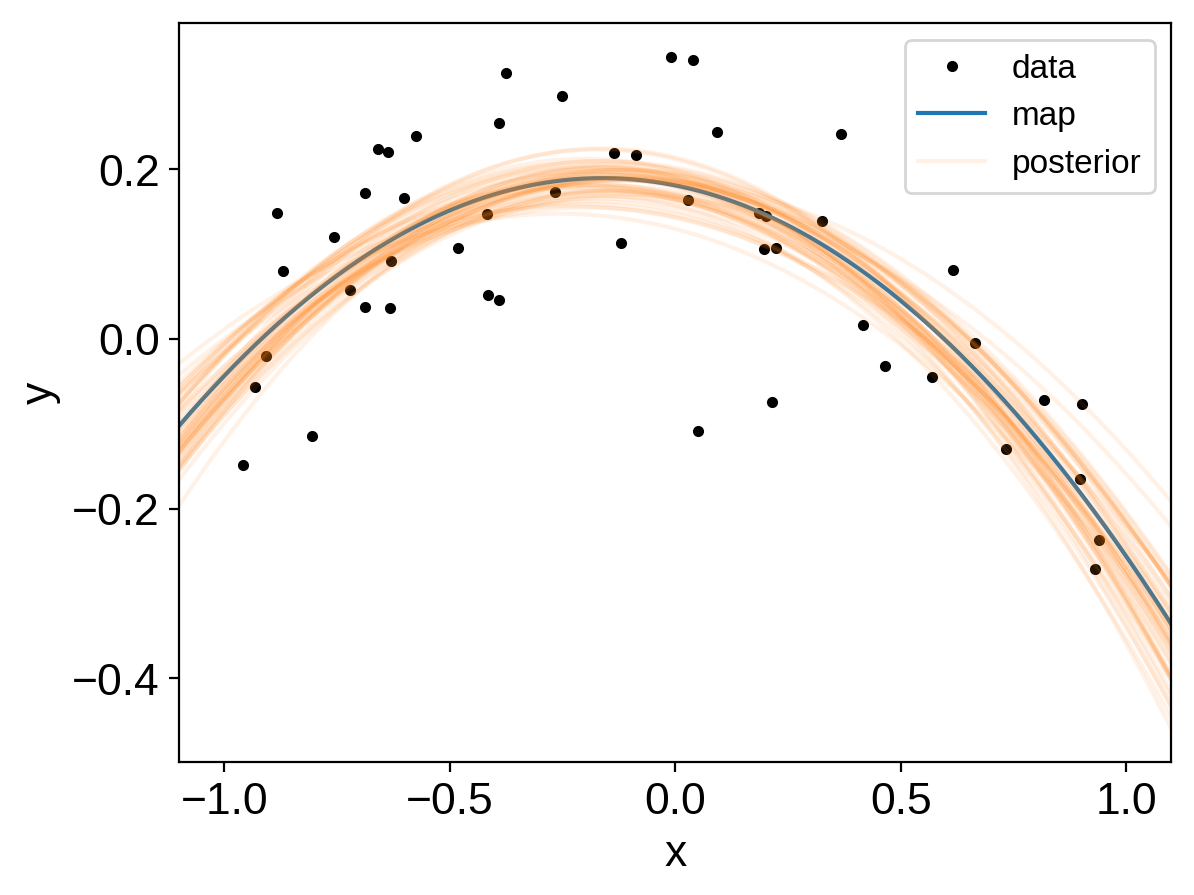
We can also combine this with exoplanet.get_samples_from_trace()
to plot this prediction for a set of samples in the trace.
samples = np.empty((50, len(x_grid)))
with model:
    y_grid = a0 + a1 * x_grid + a2 * x_grid**2
    for i, sample in enumerate(xo.get_samples_from_trace(trace, size=50)):
        samples[i] = xo.eval_in_model(y_grid, sample)

plt.plot(x, y, ".k", label="data")
plt.plot(x_grid, pred, label="map")
plt.plot(x_grid, samples[0], color="C1", alpha=0.1, label="posterior")
plt.plot(x_grid, samples[1:].T, color="C1", alpha=0.1)
plt.legend(fontsize=12)
plt.xlabel("x")
plt.ylabel("y")
plt.xlim(-1.1, 1.1);