Note
This tutorial was generated from an IPython notebook that can be downloaded here.
theano version: 1.0.4
pymc3 version: 3.7
exoplanet version: 0.2.0
In this tutorial, we will reproduce the fits to the transiting planet in the Pi Mensae system discovered by Huang et al. (2018). The data processing and model are similar to the Case study: K2-24, putting it all together tutorial, but with a few extra bits like aperture selection and de-trending.
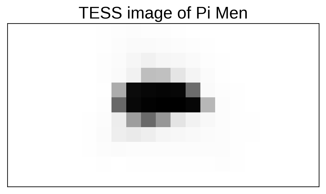
To start, we need to download the target pixel file:
import numpy as np
from astropy.io import fits
import matplotlib.pyplot as plt

tpf_url = "https://archive.stsci.edu/missions/tess/tid/s0001/0000/0002/6113/6679/tess2018206045859-s0001-0000000261136679-0120-s_tp.fits"
with fits.open(tpf_url) as hdus:
    tpf = hdus[1].data
    tpf_hdr = hdus[1].header

texp = tpf_hdr["FRAMETIM"] * tpf_hdr["NUM_FRM"]
texp /= 60.0 * 60.0 * 24.0
time = tpf["TIME"]
flux = tpf["FLUX"]
m = np.any(np.isfinite(flux), axis=(1, 2)) & (tpf["QUALITY"] == 0)
ref_time = 0.5 * (np.min(time[m])+np.max(time[m]))
time = np.ascontiguousarray(time[m] - ref_time, dtype=np.float64)
flux = np.ascontiguousarray(flux[m], dtype=np.float64)

mean_img = np.median(flux, axis=0)
plt.imshow(mean_img.T, cmap="gray_r")
plt.title("TESS image of Pi Men")
plt.xticks([])
plt.yticks([]);
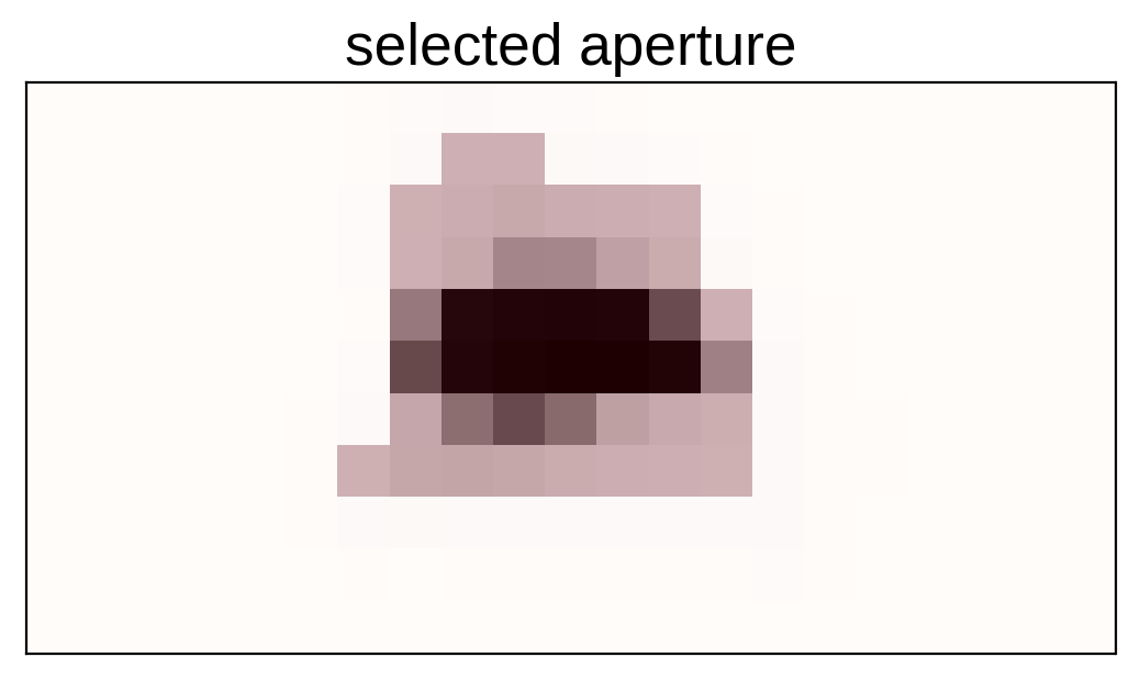
Next, we’ll select an aperture using a hacky method that tries to minimizes the windowed scatter in the lightcurve (something like the CDPP).
from scipy.signal import savgol_filter

# Sort the pixels by median brightness
order = np.argsort(mean_img.flatten())[::-1]

# A function to estimate the windowed scatter in a lightcurve
def estimate_scatter_with_mask(mask):
    f = np.sum(flux[:, mask], axis=-1)
    smooth = savgol_filter(f, 1001, polyorder=5)
    return 1e6 * np.sqrt(np.median((f / smooth - 1)**2))

# Loop over pixels ordered by brightness and add them one-by-one
# to the aperture
masks, scatters = [], []
for i in range(10, 100):
    msk = np.zeros_like(mean_img, dtype=bool)
    msk[np.unravel_index(order[:i], mean_img.shape)] = True
    scatter = estimate_scatter_with_mask(msk)
    masks.append(msk)
    scatters.append(scatter)

# Choose the aperture that minimizes the scatter
pix_mask = masks[np.argmin(scatters)]

# Plot the selected aperture
plt.imshow(mean_img.T, cmap="gray_r")
plt.imshow(pix_mask.T, cmap="Reds", alpha=0.3)
plt.title("selected aperture")
plt.xticks([])
plt.yticks([]);
This aperture produces the following light curve:
plt.figure(figsize=(10, 5))
sap_flux = np.sum(flux[:, pix_mask], axis=-1)
sap_flux = (sap_flux / np.median(sap_flux) - 1) * 1e3
plt.plot(time, sap_flux, "k")
plt.xlabel("time [days]")
plt.ylabel("relative flux [ppt]")
plt.title("raw light curve")
plt.xlim(time.min(), time.max());
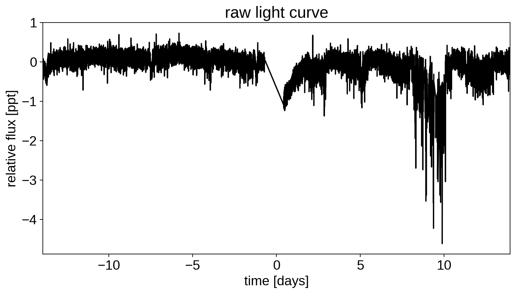
This doesn’t look terrible, but we’re still going to want to de-trend it a little bit. We’ll use “pixel-level deconvolution” (PLD) to de-trend following the method used by Everest. Specifically, we’ll use first order PLD plus the top few PCA components of the second order PLD basis.
# Build the first order PLD basis
X_pld = np.reshape(flux[:, pix_mask], (len(flux), -1))
X_pld = X_pld / np.sum(flux[:, pix_mask], axis=-1)[:, None]

# Build the second order PLD basis and run PCA to reduce the number of dimensions
X2_pld = np.reshape(X_pld[:, None, :] * X_pld[:, :, None], (len(flux), -1))
U, _, _ = np.linalg.svd(X2_pld, full_matrices=False)
X2_pld = U[:, :X_pld.shape[1]]

# Construct the design matrix and fit for the PLD model
X_pld = np.concatenate((np.ones((len(flux), 1)), X_pld, X2_pld), axis=-1)
XTX = np.dot(X_pld.T, X_pld)
w_pld = np.linalg.solve(XTX, np.dot(X_pld.T, sap_flux))
pld_flux = np.dot(X_pld, w_pld)

# Plot the de-trended light curve
plt.figure(figsize=(10, 5))
plt.plot(time, sap_flux-pld_flux, "k")
plt.xlabel("time [days]")
plt.ylabel("de-trended flux [ppt]")
plt.title("initial de-trended light curve")
plt.xlim(time.min(), time.max());
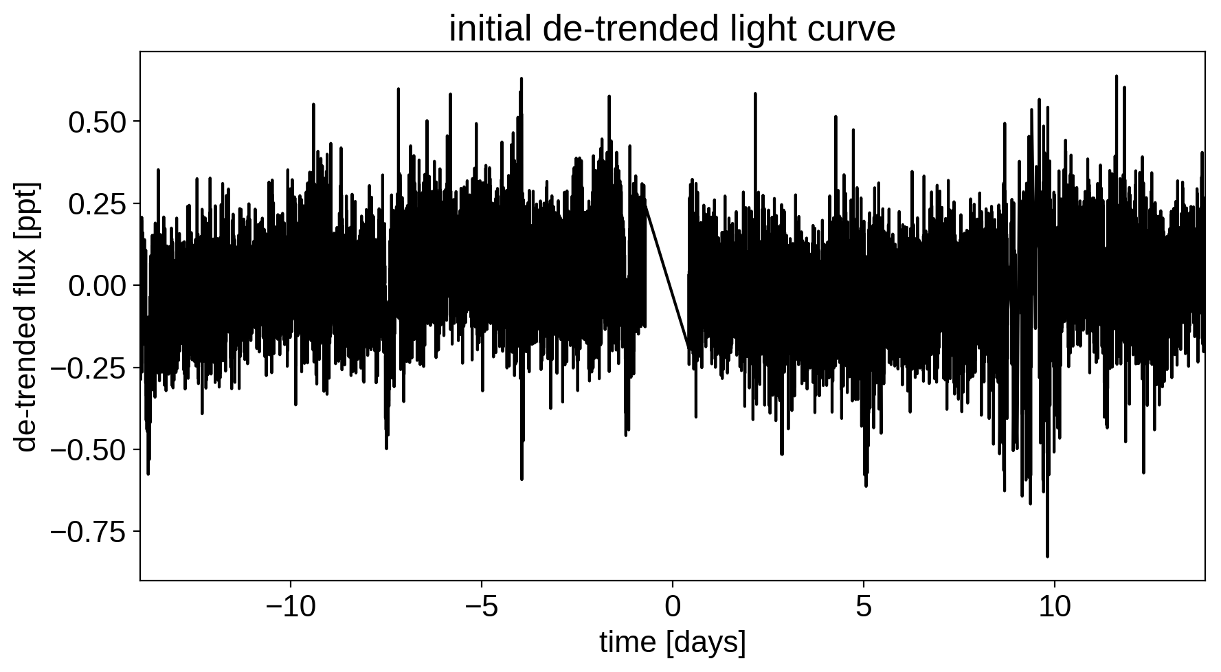
That looks better.
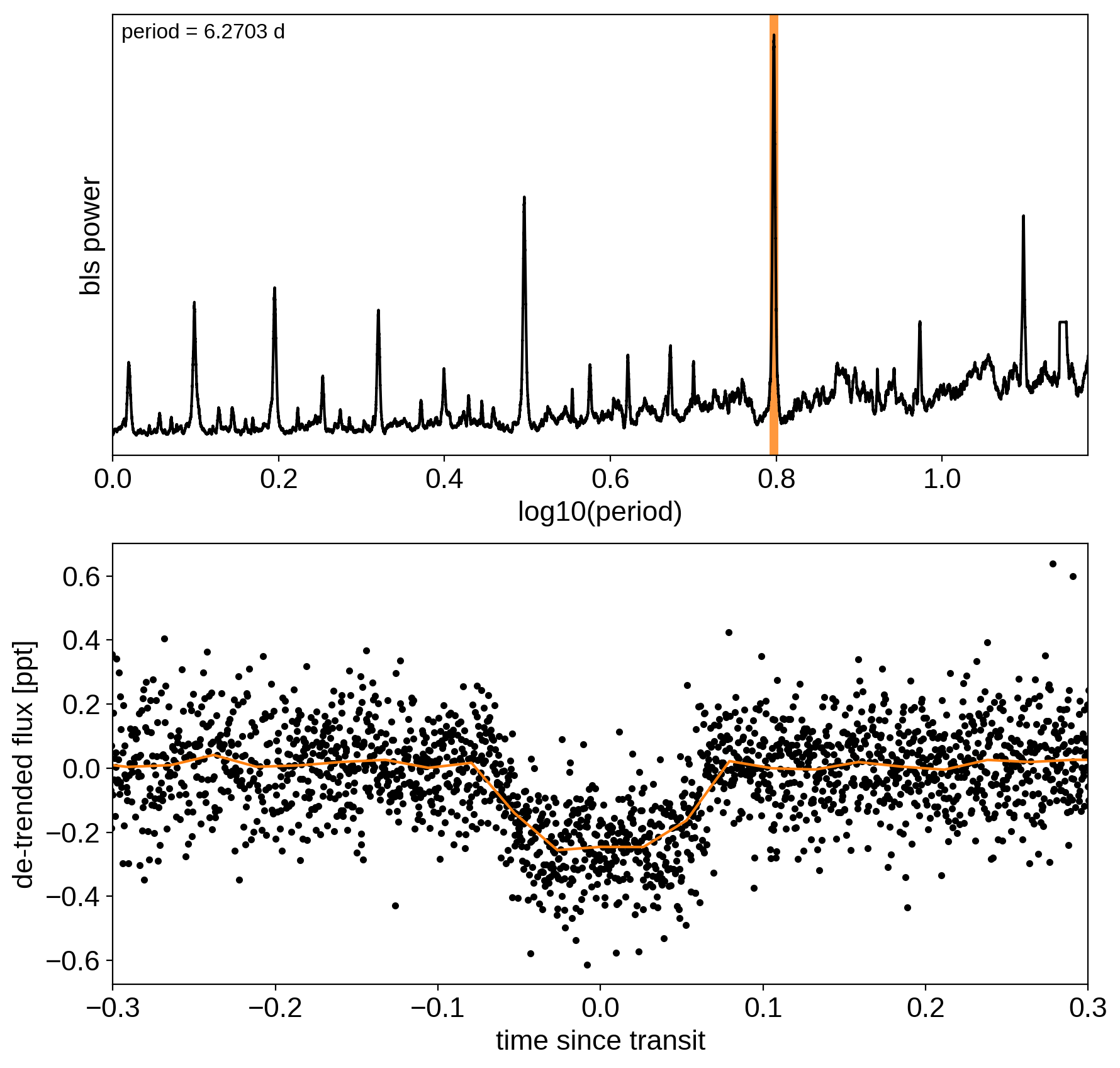
Now, let’s use the box least squares periodogram from AstroPy (Note: you’ll need AstroPy v3.1 or more recent to use this feature) to estimate the period, phase, and depth of the transit.
from astropy.stats import BoxLeastSquares

period_grid = np.exp(np.linspace(np.log(1), np.log(15), 50000))

bls = BoxLeastSquares(time, sap_flux - pld_flux)
bls_power = bls.power(period_grid, 0.1, oversample=20)

# Save the highest peak as the planet candidate
index = np.argmax(bls_power.power)
bls_period = bls_power.period[index]
bls_t0 = bls_power.transit_time[index]
bls_depth = bls_power.depth[index]
transit_mask = bls.transit_mask(time, bls_period, 0.2, bls_t0)

fig, axes = plt.subplots(2, 1, figsize=(10, 10))

# Plot the periodogram
ax = axes[0]
ax.axvline(np.log10(bls_period), color="C1", lw=5, alpha=0.8)
ax.plot(np.log10(bls_power.period), bls_power.power, "k")
ax.annotate("period = {0:.4f} d".format(bls_period),
            (0, 1), xycoords="axes fraction",
            xytext=(5, -5), textcoords="offset points",
            va="top", ha="left", fontsize=12)
ax.set_ylabel("bls power")
ax.set_yticks([])
ax.set_xlim(np.log10(period_grid.min()), np.log10(period_grid.max()))
ax.set_xlabel("log10(period)")

# Plot the folded transit
ax = axes[1]
x_fold = (time - bls_t0 + 0.5*bls_period)%bls_period - 0.5*bls_period
m = np.abs(x_fold) < 0.4
ax.plot(x_fold[m], sap_flux[m] - pld_flux[m], ".k")

# Overplot the phase binned light curve
bins = np.linspace(-0.41, 0.41, 32)
denom, _ = np.histogram(x_fold, bins)
num, _ = np.histogram(x_fold, bins, weights=sap_flux - pld_flux)
denom[num == 0] = 1.0
ax.plot(0.5*(bins[1:] + bins[:-1]), num / denom, color="C1")

ax.set_xlim(-0.3, 0.3)
ax.set_ylabel("de-trended flux [ppt]")
ax.set_xlabel("time since transit");
Now that we know where the transits are, it’s generally good practice to de-trend the data one more time with the transits masked so that the de-trending doesn’t overfit the transits. Let’s do that.
m = ~transit_mask
XTX = np.dot(X_pld[m].T, X_pld[m])
w_pld = np.linalg.solve(XTX, np.dot(X_pld[m].T, sap_flux[m]))
pld_flux = np.dot(X_pld, w_pld)

x = np.ascontiguousarray(time, dtype=np.float64)
y = np.ascontiguousarray(sap_flux-pld_flux, dtype=np.float64)

plt.figure(figsize=(10, 5))
plt.plot(time, y, "k")
plt.xlabel("time [days]")
plt.ylabel("de-trended flux [ppt]")
plt.title("final de-trended light curve")
plt.xlim(time.min(), time.max());
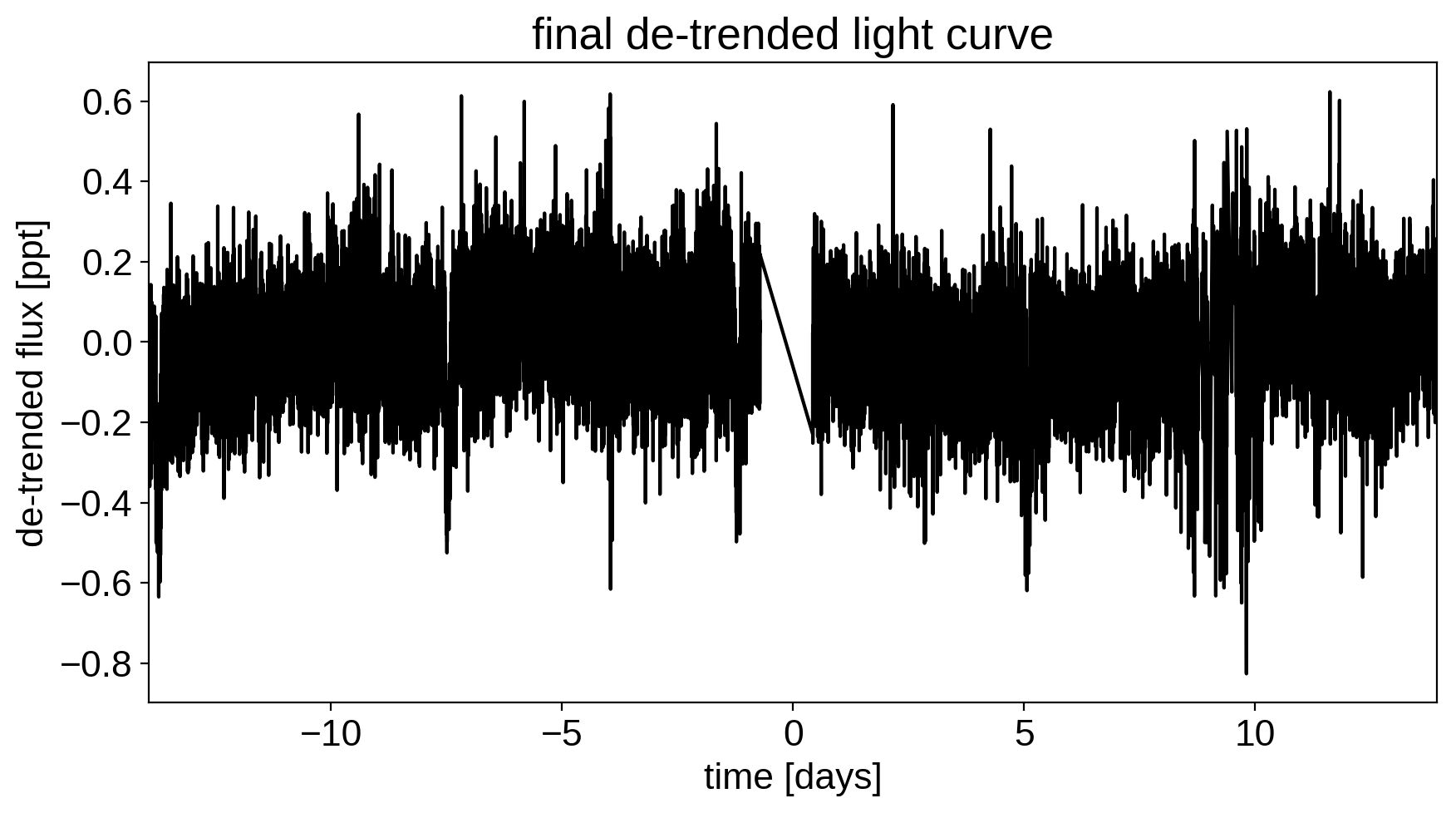
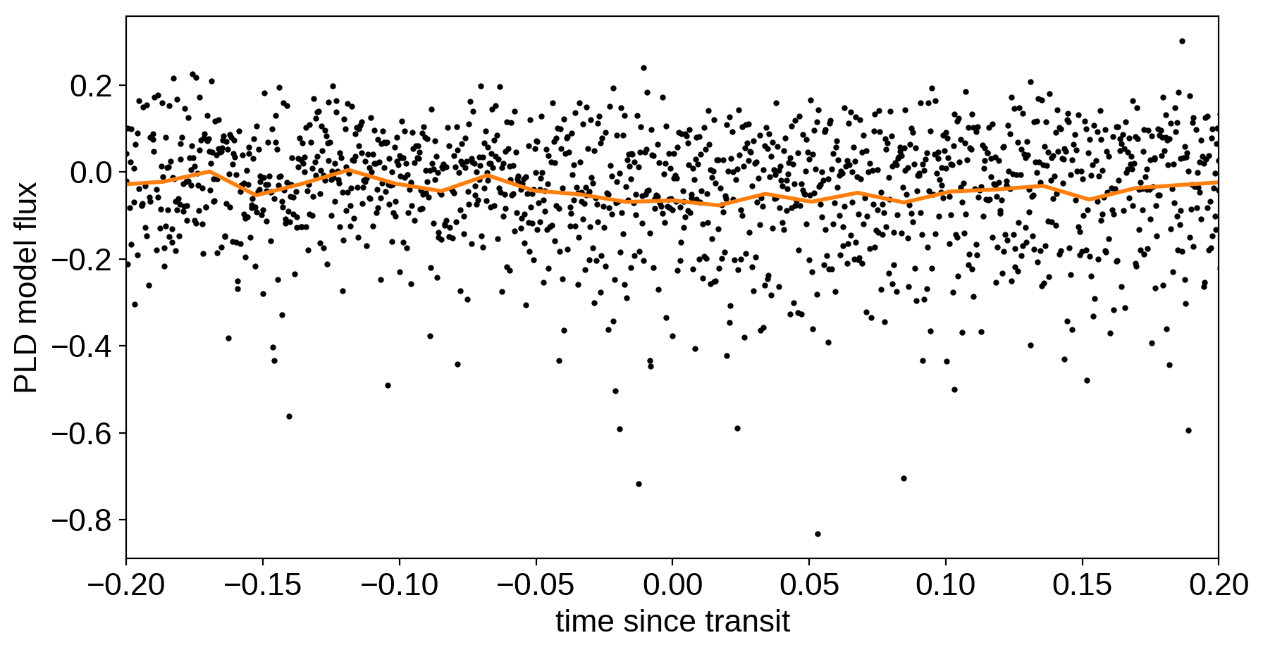
To confirm that we didn’t overfit the transit, we can look at the folded light curve for the PLD model near trasit. This shouldn’t have any residual transit signal, and that looks correct here:
plt.figure(figsize=(10, 5))

x_fold = (x - bls_t0 + 0.5*bls_period) % bls_period - 0.5*bls_period
m = np.abs(x_fold) < 0.3
plt.plot(x_fold[m], pld_flux[m], ".k", ms=4)

bins = np.linspace(-0.5, 0.5, 60)
denom, _ = np.histogram(x_fold, bins)
num, _ = np.histogram(x_fold, bins, weights=pld_flux)
denom[num == 0] = 1.0
plt.plot(0.5*(bins[1:] + bins[:-1]), num / denom, color="C1", lw=2)
plt.xlim(-0.2, 0.2)
plt.xlabel("time since transit")
plt.ylabel("PLD model flux");
The transit model, initialization, and sampling are all nearly the same as the one in Case study: K2-24, putting it all together, but we’ll use a more informative prior on eccentricity.
import exoplanet as xo
import pymc3 as pm
import theano.tensor as tt

def build_model(mask=None, start=None):
    if mask is None:
        mask = np.ones(len(x), dtype=bool)
    with pm.Model() as model:

        # Parameters for the stellar properties
        mean = pm.Normal("mean", mu=0.0, sd=10.0)
        u_star = xo.distributions.QuadLimbDark("u_star")

        # Stellar parameters from Huang et al (2018)
        M_star_huang = 1.094, 0.039
        R_star_huang = 1.10, 0.023
        BoundedNormal = pm.Bound(pm.Normal, lower=0, upper=3)
        m_star = BoundedNormal("m_star", mu=M_star_huang[0], sd=M_star_huang[1])
        r_star = BoundedNormal("r_star", mu=R_star_huang[0], sd=R_star_huang[1])

        # Orbital parameters for the planets
        logP = pm.Normal("logP", mu=np.log(bls_period), sd=1)
        t0 = pm.Normal("t0", mu=bls_t0, sd=1)
        b = xo.distributions.UnitUniform("b")
        logr = pm.Normal("logr", sd=1.0,
                         mu=0.5*np.log(1e-3*np.array(bls_depth))+np.log(R_star_huang[0]))
        r_pl = pm.Deterministic("r_pl", tt.exp(logr))
        ror = pm.Deterministic("ror", r_pl / r_star)

        # This is the eccentricity prior from Kipping (2013):
        # https://arxiv.org/abs/1306.4982
        BoundedBeta = pm.Bound(pm.Beta, lower=0, upper=1-1e-5)
        ecc = BoundedBeta("ecc", alpha=0.867, beta=3.03, testval=0.1)
        omega = xo.distributions.Angle("omega")

        # Transit jitter & GP parameters
        logs2 = pm.Normal("logs2", mu=np.log(np.var(y[mask])), sd=10)
        logw0_guess = np.log(2*np.pi/10)
        logw0 = pm.Normal("logw0", mu=logw0_guess, sd=10)

        # We'll parameterize using the maximum power (S_0 * w_0^4) instead of
        # S_0 directly because this removes some of the degeneracies between
        # S_0 and omega_0
        logpower = pm.Normal("logpower",
                             mu=np.log(np.var(y[mask]))+4*logw0_guess,
                             sd=10)
        logS0 = pm.Deterministic("logS0", logpower - 4 * logw0)

        # Tracking planet parameters
        period = pm.Deterministic("period", tt.exp(logP))

        # Orbit model
        orbit = xo.orbits.KeplerianOrbit(
            r_star=r_star, m_star=m_star,
            period=period, t0=t0, b=b,
            ecc=ecc, omega=omega)

        # Compute the model light curve using starry
        light_curves = xo.LimbDarkLightCurve(u_star).get_light_curve(
            orbit=orbit, r=r_pl, t=x[mask], texp=texp)*1e3
        light_curve = pm.math.sum(light_curves, axis=-1) + mean
        pm.Deterministic("light_curves", light_curves)

        # GP model for the light curve
        kernel = xo.gp.terms.SHOTerm(log_S0=logS0, log_w0=logw0, Q=1/np.sqrt(2))
        gp = xo.gp.GP(kernel, x[mask], tt.exp(logs2) + tt.zeros(mask.sum()), J=2)
        pm.Potential("transit_obs", gp.log_likelihood(y[mask] - light_curve))
        pm.Deterministic("gp_pred", gp.predict())

        # Fit for the maximum a posteriori parameters, I've found that I can get
        # a better solution by trying different combinations of parameters in turn
        if start is None:
            start = model.test_point
        map_soln = xo.optimize(start=start, vars=[logs2, logpower, logw0])
        map_soln = xo.optimize(start=map_soln, vars=[logr])
        map_soln = xo.optimize(start=map_soln, vars=[b])
        map_soln = xo.optimize(start=map_soln, vars=[logP, t0])
        map_soln = xo.optimize(start=map_soln, vars=[u_star])
        map_soln = xo.optimize(start=map_soln, vars=[logr])
        map_soln = xo.optimize(start=map_soln, vars=[b])
        map_soln = xo.optimize(start=map_soln, vars=[ecc, omega])
        map_soln = xo.optimize(start=map_soln, vars=[mean])
        map_soln = xo.optimize(start=map_soln, vars=[logs2, logpower, logw0])
        map_soln = xo.optimize(start=map_soln)

    return model, map_soln

model0, map_soln0 = build_model()
optimizing logp for variables: ['logw0', 'logpower', 'logs2']
message: Optimization terminated successfully.
logp: 12376.808570986894 -> 12639.99697023041
optimizing logp for variables: ['logr']
message: Optimization terminated successfully.
logp: 12639.99697023041 -> 12678.437541150912
optimizing logp for variables: ['b_logodds__']
message: Optimization terminated successfully.
logp: 12678.437541150905 -> 12766.212035563016
optimizing logp for variables: ['t0', 'logP']
message: Desired error not necessarily achieved due to precision loss.
logp: 12766.212035563016 -> 12775.28026595461
optimizing logp for variables: ['u_star_quadlimbdark__']
message: Optimization terminated successfully.
logp: 12775.2802659546 -> 12785.944976507275
optimizing logp for variables: ['logr']
message: Optimization terminated successfully.
logp: 12785.944976507275 -> 12808.533811467807
optimizing logp for variables: ['b_logodds__']
message: Optimization terminated successfully.
logp: 12808.533811467814 -> 12810.245024497966
optimizing logp for variables: ['omega_angle__', 'ecc_interval__']
message: Optimization terminated successfully.
logp: 12810.245024497966 -> 12830.745429465525
optimizing logp for variables: ['mean']
message: Optimization terminated successfully.
logp: 12830.745429465522 -> 12830.776889877343
optimizing logp for variables: ['logw0', 'logpower', 'logs2']
message: Optimization terminated successfully.
logp: 12830.776889877343 -> 12841.612045223597
optimizing logp for variables: ['logpower', 'logw0', 'logs2', 'omega_angle__', 'ecc_interval__', 'logr', 'b_logodds__', 't0', 'logP', 'r_star_interval__', 'm_star_interval__', 'u_star_quadlimbdark__', 'mean']
message: Desired error not necessarily achieved due to precision loss.
logp: 12841.612045223583 -> 13051.73491486121
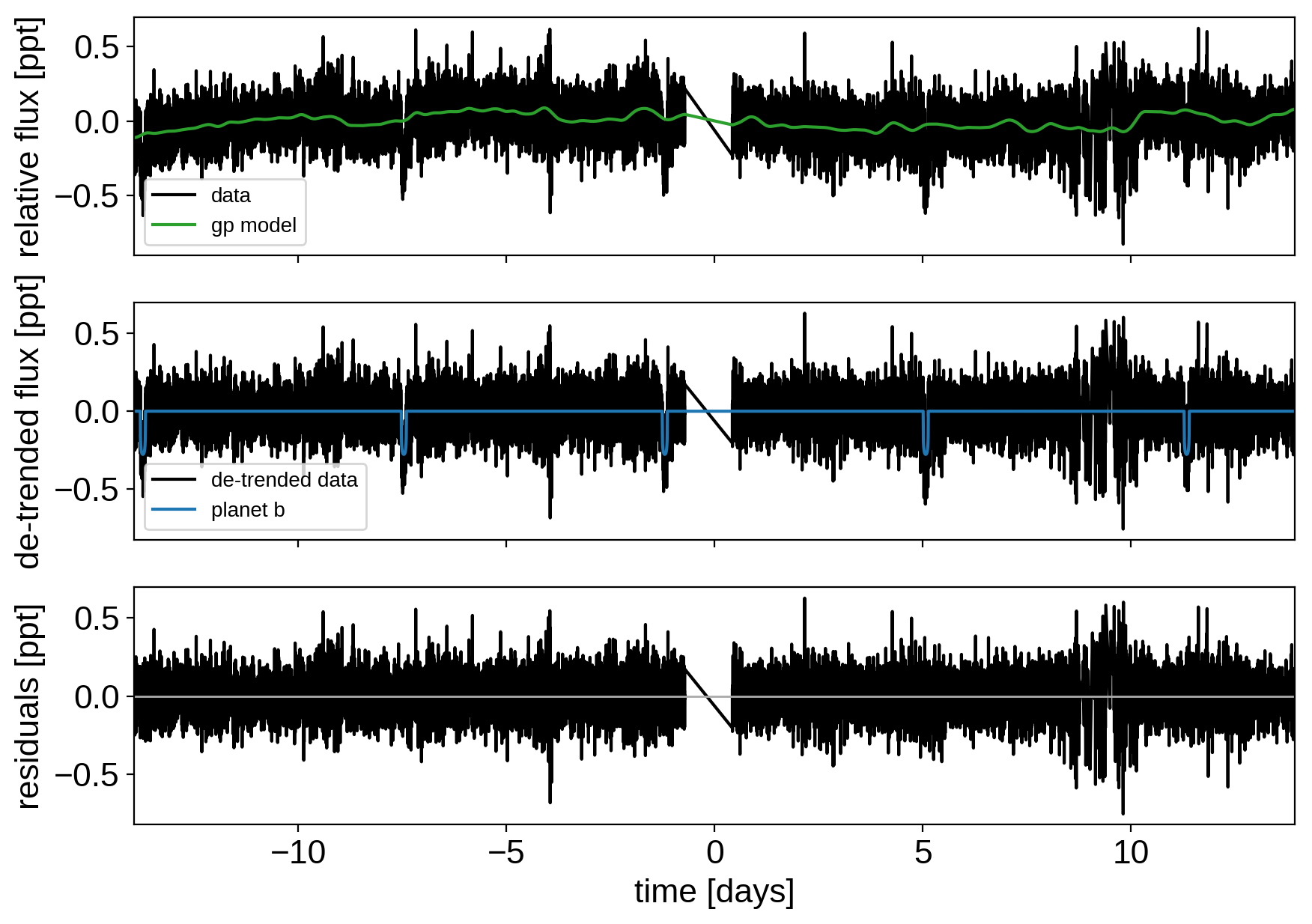
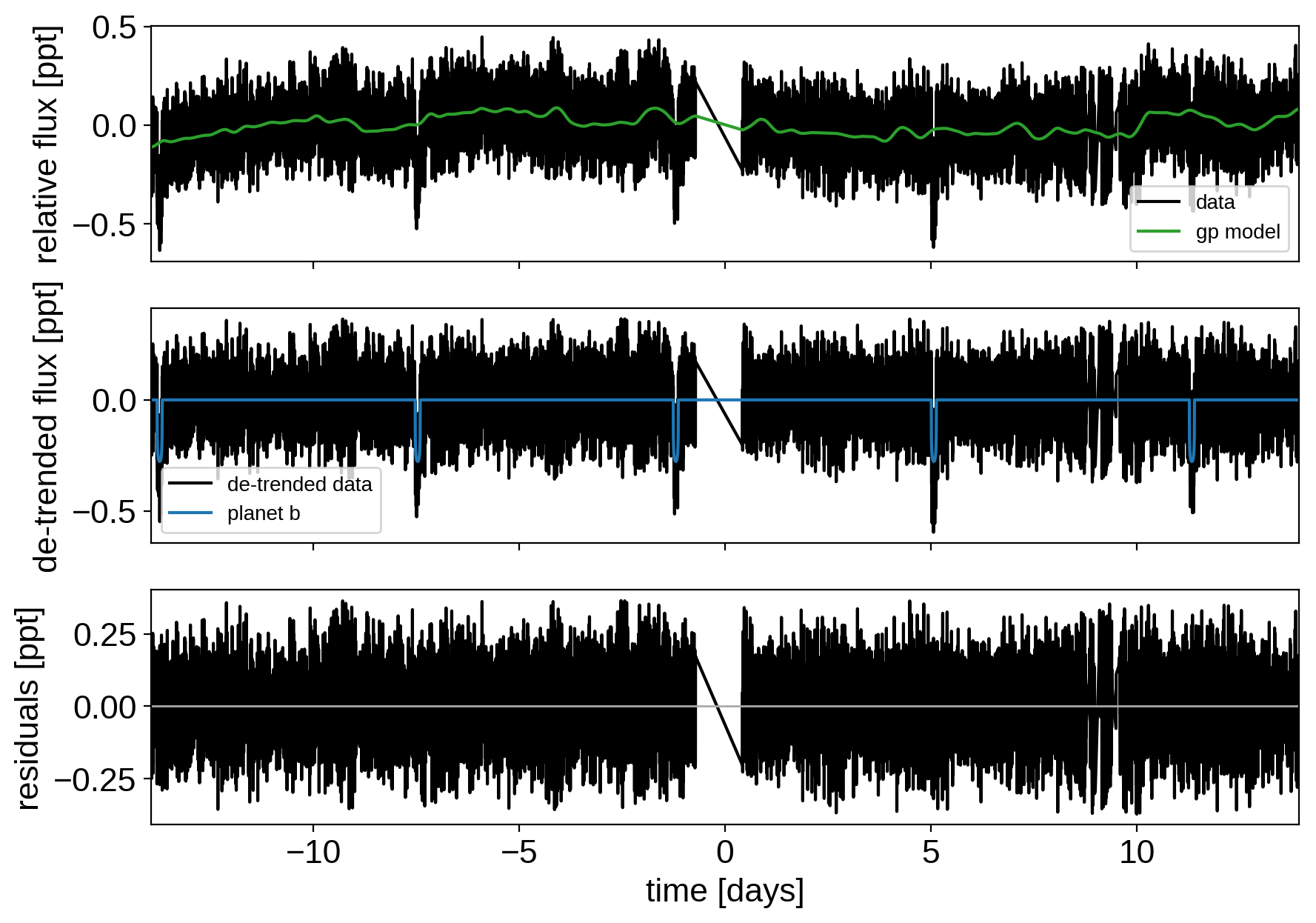
Here’s how we plot the initial light curve model:
def plot_light_curve(soln, mask=None):
    if mask is None:
        mask = np.ones(len(x), dtype=bool)

    fig, axes = plt.subplots(3, 1, figsize=(10, 7), sharex=True)

    ax = axes[0]
    ax.plot(x[mask], y[mask], "k", label="data")
    gp_mod = soln["gp_pred"] + soln["mean"]
    ax.plot(x[mask], gp_mod, color="C2", label="gp model")
    ax.legend(fontsize=10)
    ax.set_ylabel("relative flux [ppt]")

    ax = axes[1]
    ax.plot(x[mask], y[mask] - gp_mod, "k", label="de-trended data")
    for i, l in enumerate("b"):
        mod = soln["light_curves"][:, i]
        ax.plot(x[mask], mod, label="planet {0}".format(l))
    ax.legend(fontsize=10, loc=3)
    ax.set_ylabel("de-trended flux [ppt]")

    ax = axes[2]
    mod = gp_mod + np.sum(soln["light_curves"], axis=-1)
    ax.plot(x[mask], y[mask] - mod, "k")
    ax.axhline(0, color="#aaaaaa", lw=1)
    ax.set_ylabel("residuals [ppt]")
    ax.set_xlim(x[mask].min(), x[mask].max())
    ax.set_xlabel("time [days]")

    return fig

plot_light_curve(map_soln0);
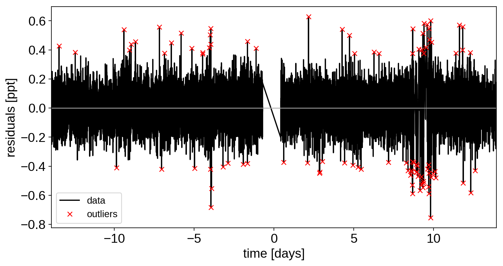
As in the Case study: K2-24, putting it all together tutorial, we can do some sigma clipping to remove significant outliers.
mod = map_soln0["gp_pred"] + map_soln0["mean"] + np.sum(map_soln0["light_curves"], axis=-1)
resid = y - mod
rms = np.sqrt(np.median(resid**2))
mask = np.abs(resid) < 5 * rms

plt.figure(figsize=(10, 5))
plt.plot(x, resid, "k", label="data")
plt.plot(x[~mask], resid[~mask], "xr", label="outliers")
plt.axhline(0, color="#aaaaaa", lw=1)
plt.ylabel("residuals [ppt]")
plt.xlabel("time [days]")
plt.legend(fontsize=12, loc=3)
plt.xlim(x.min(), x.max());
And then we re-build the model using the data without outliers.
model, map_soln = build_model(mask, map_soln0)
plot_light_curve(map_soln, mask);
optimizing logp for variables: ['logw0', 'logpower', 'logs2']
message: Optimization terminated successfully.
logp: 13706.240110607976 -> 13737.199586335446
optimizing logp for variables: ['logr']
message: Optimization terminated successfully.
logp: 13737.199586335446 -> 13737.21973823953
optimizing logp for variables: ['b_logodds__']
message: Optimization terminated successfully.
logp: 13737.219738239526 -> 13737.220611244695
optimizing logp for variables: ['t0', 'logP']
message: Optimization terminated successfully.
logp: 13737.220611244695 -> 13737.22944778266
optimizing logp for variables: ['u_star_quadlimbdark__']
message: Optimization terminated successfully.
logp: 13737.229447782656 -> 13737.253296045787
optimizing logp for variables: ['logr']
message: Optimization terminated successfully.
logp: 13737.253296045787 -> 13737.256456122668
optimizing logp for variables: ['b_logodds__']
message: Desired error not necessarily achieved due to precision loss.
logp: 13737.256456122665 -> 13737.265293068196
optimizing logp for variables: ['omega_angle__', 'ecc_interval__']
message: Optimization terminated successfully.
logp: 13737.265293068192 -> 13737.265332658291
optimizing logp for variables: ['mean']
message: Optimization terminated successfully.
logp: 13737.265332658284 -> 13737.26848380823
optimizing logp for variables: ['logw0', 'logpower', 'logs2']
message: Optimization terminated successfully.
logp: 13737.26848380823 -> 13737.268486665855
optimizing logp for variables: ['logpower', 'logw0', 'logs2', 'omega_angle__', 'ecc_interval__', 'logr', 'b_logodds__', 't0', 'logP', 'r_star_interval__', 'm_star_interval__', 'u_star_quadlimbdark__', 'mean']
message: Desired error not necessarily achieved due to precision loss.
logp: 13737.268486665851 -> 13737.280285382387
Now that we have the model, we can sample it using a
exoplanet.PyMC3Sampler:
np.random.seed(42)
sampler = xo.PyMC3Sampler(start=200, window=100, finish=500, chains=4)
with model:
    burnin = sampler.tune(tune=4500, start=map_soln,
                          step_kwargs=dict(target_accept=0.9))
Sampling 4 chains: 100%|██████████| 808/808 [06:17<00:00,  1.99s/draws]
Sampling 4 chains: 100%|██████████| 408/408 [02:55<00:00,  1.40s/draws]
Sampling 4 chains: 100%|██████████| 808/808 [05:20<00:00,  1.29s/draws]
Sampling 4 chains: 100%|██████████| 1608/1608 [06:48<00:00,  1.11draws/s]
Sampling 4 chains: 100%|██████████| 3208/3208 [15:02<00:00,  3.56draws/s]
Sampling 4 chains: 100%|██████████| 11208/11208 [50:16<00:00,  1.12draws/s]
Sampling 4 chains: 100%|██████████| 2008/2008 [10:05<00:00,  1.00s/draws]
with model:
    trace = sampler.sample(draws=3000)
Multiprocess sampling (4 chains in 4 jobs)
NUTS: [logpower, logw0, logs2, omega, ecc, logr, b, t0, logP, r_star, m_star, u_star, mean]
Sampling 4 chains: 100%|██████████| 12000/12000 [50:10<00:00,  1.07draws/s]
The number of effective samples is smaller than 25% for some parameters.
pm.summary(trace, varnames=["logw0", "logpower", "logs2", "omega", "ecc", "r_pl", "b", "t0", "logP", "r_star", "m_star", "u_star", "mean"])
| mean | sd | mc_error | hpd_2.5 | hpd_97.5 | n_eff | Rhat | |
|---|---|---|---|---|---|---|---|
| logw0 | 1.178053 | 0.135057 | 1.507431e-03 | 0.912220 | 1.438115 | 8923.066852 | 1.000072 |
| logpower | -2.105123 | 0.315618 | 3.327547e-03 | -2.722754 | -1.502855 | 10290.298819 | 1.000109 |
| logs2 | -4.382782 | 0.010432 | 8.981302e-05 | -4.403634 | -4.362955 | 11374.945224 | 0.999934 |
| omega | 0.649544 | 1.706494 | 3.621051e-02 | -2.781730 | 3.137032 | 2185.933177 | 1.000017 |
| ecc | 0.197019 | 0.142911 | 3.549473e-03 | 0.000027 | 0.481502 | 1491.031160 | 1.002402 |
| r_pl | 0.017266 | 0.000677 | 1.637331e-05 | 0.016008 | 0.018576 | 1435.832816 | 1.002052 |
| b | 0.412518 | 0.212245 | 4.841889e-03 | 0.000093 | 0.725954 | 1746.875612 | 1.001746 |
| t0 | -1.197358 | 0.000670 | 1.212194e-05 | -1.198718 | -1.196067 | 2428.179591 | 1.000265 |
| logP | 1.835412 | 0.000070 | 8.432120e-07 | 1.835268 | 1.835534 | 7139.574981 | 1.000379 |
| r_star | 1.098560 | 0.023223 | 2.536181e-04 | 1.051926 | 1.143934 | 8395.167716 | 1.000064 |
| m_star | 1.095535 | 0.038344 | 3.810941e-04 | 1.021626 | 1.171791 | 11795.648699 | 0.999966 |
| u_star__0 | 0.202535 | 0.174174 | 3.037353e-03 | 0.000004 | 0.542884 | 2612.694466 | 1.001118 |
| u_star__1 | 0.453342 | 0.276940 | 4.524016e-03 | -0.100696 | 0.939617 | 3242.872737 | 1.001691 |
| mean | -0.001276 | 0.009119 | 9.434227e-05 | -0.019037 | 0.017051 | 9504.052864 | 0.999868 |
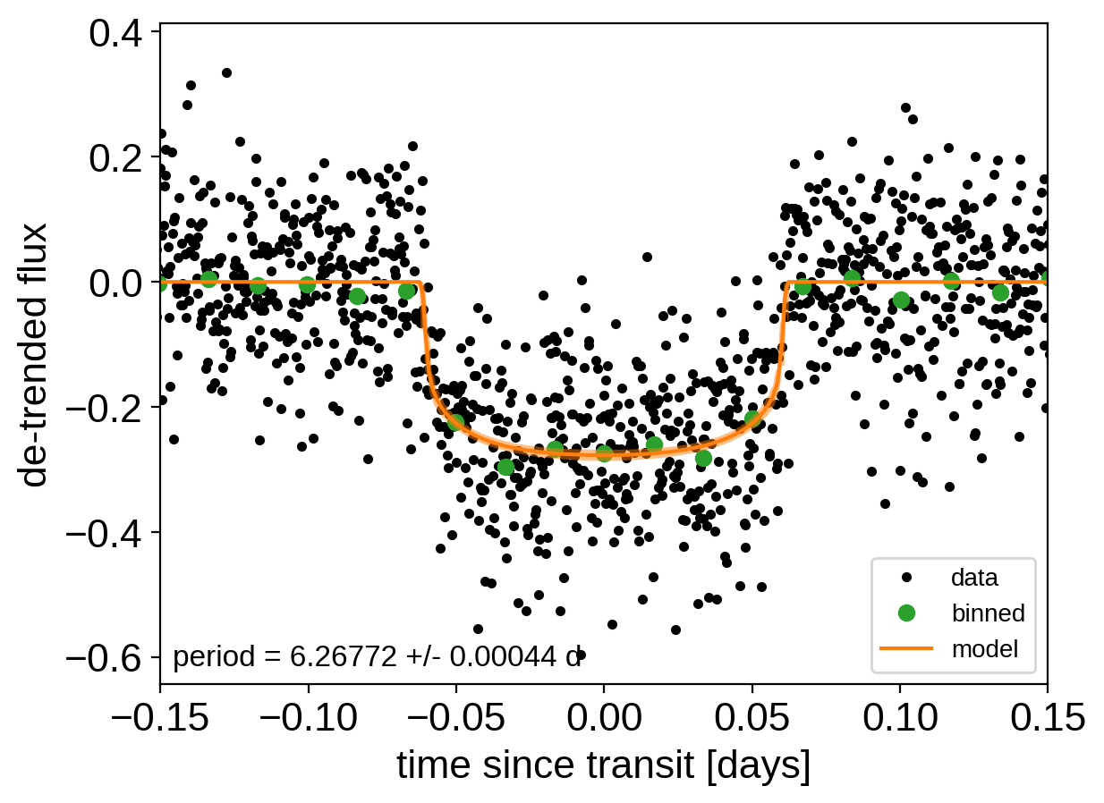
After sampling, we can make the usual plots. First, let’s look at the folded light curve plot:
# Compute the GP prediction
gp_mod = np.median(trace["gp_pred"] + trace["mean"][:, None], axis=0)

# Get the posterior median orbital parameters
p = np.median(trace["period"])
t0 = np.median(trace["t0"])

# Plot the folded data
x_fold = (x[mask] - t0 + 0.5*p) % p - 0.5*p
plt.plot(x_fold, y[mask] - gp_mod, ".k", label="data", zorder=-1000)

# Overplot the phase binned light curve
bins = np.linspace(-0.41, 0.41, 50)
denom, _ = np.histogram(x_fold, bins)
num, _ = np.histogram(x_fold, bins, weights=y[mask])
denom[num == 0] = 1.0
plt.plot(0.5*(bins[1:] + bins[:-1]), num / denom, "o", color="C2",
         label="binned")

# Plot the folded model
inds = np.argsort(x_fold)
inds = inds[np.abs(x_fold)[inds] < 0.3]
pred = trace["light_curves"][:, inds, 0]
pred = np.percentile(pred, [16, 50, 84], axis=0)
plt.plot(x_fold[inds], pred[1], color="C1", label="model")
art = plt.fill_between(x_fold[inds], pred[0], pred[2], color="C1", alpha=0.5,
                       zorder=1000)
art.set_edgecolor("none")

# Annotate the plot with the planet's period
txt = "period = {0:.5f} +/- {1:.5f} d".format(
    np.mean(trace["period"]), np.std(trace["period"]))
plt.annotate(txt, (0, 0), xycoords="axes fraction",
             xytext=(5, 5), textcoords="offset points",
             ha="left", va="bottom", fontsize=12)

plt.legend(fontsize=10, loc=4)
plt.xlim(-0.5*p, 0.5*p)
plt.xlabel("time since transit [days]")
plt.ylabel("de-trended flux")
plt.xlim(-0.15, 0.15);
And a corner plot of some of the key parameters:
import corner
import astropy.units as u
varnames = ["period", "b", "ecc", "r_pl"]
samples = pm.trace_to_dataframe(trace, varnames=varnames)

# Convert the radius to Earth radii
samples["r_pl"] = (np.array(samples["r_pl"]) * u.R_sun).to(u.R_earth).value

corner.corner(
    samples[["period", "r_pl", "b", "ecc"]],
    labels=["period [days]", "radius [Earth radii]", "impact param", "eccentricity"]);
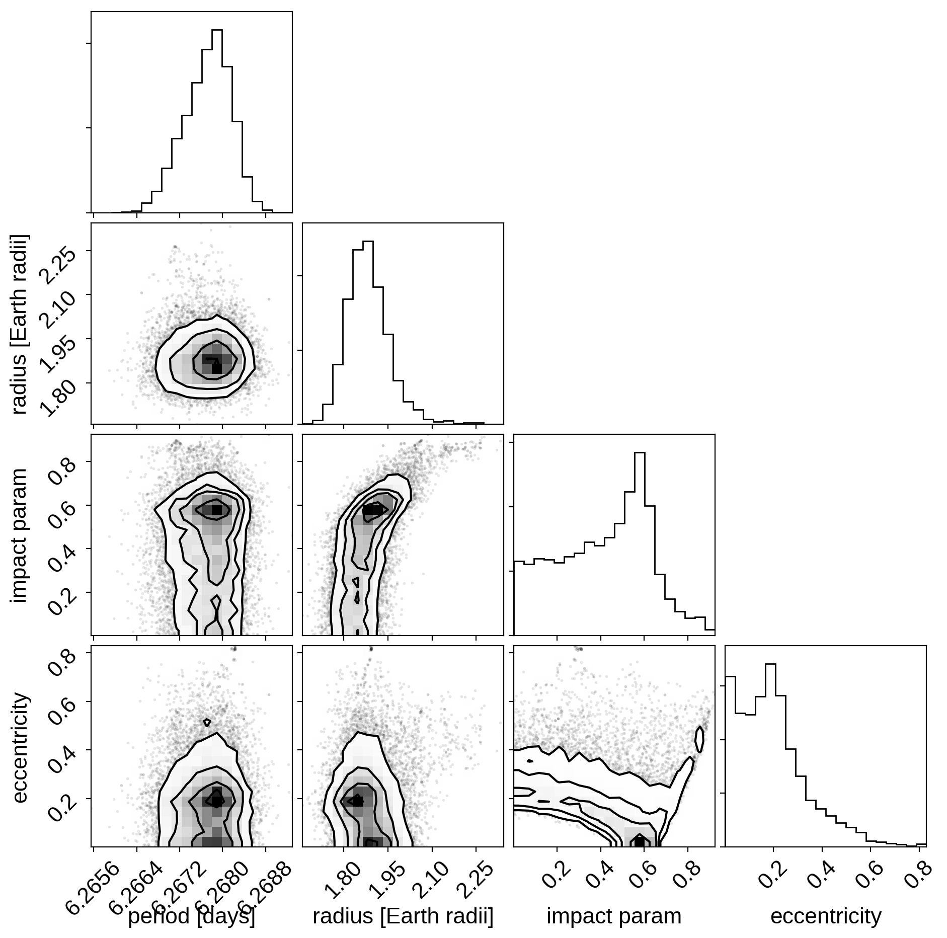
These all seem consistent with the previously published values and an earlier inconsistency between this radius measurement and the literature has been resolved by fixing a bug in exoplanet.
As described in the Citing exoplanet & its dependencies tutorial, we can use
exoplanet.citations.get_citations_for_model() to construct an
acknowledgement and BibTeX listing that includes the relevant citations
for this model.
with model:
    txt, bib = xo.citations.get_citations_for_model()
print(txt)
This research made use of textsf{exoplanet} citep{exoplanet} and its
dependencies citep{exoplanet:astropy13, exoplanet:astropy18,
exoplanet:exoplanet, exoplanet:foremanmackey17, exoplanet:foremanmackey18,
exoplanet:kipping13, exoplanet:luger18, exoplanet:pymc3, exoplanet:theano}.
print("\n".join(bib.splitlines()[:10]) + "\n...")
@misc{exoplanet:exoplanet,
  author = {Dan Foreman-Mackey and
            Geert Barentsen and
            Tom Barclay},
   title = {dfm/exoplanet: exoplanet v0.1.6},
   month = apr,
    year = 2019,
     doi = {10.5281/zenodo.2651251},
     url = {https://doi.org/10.5281/zenodo.2651251}
...