Note

This tutorial was generated from an IPython notebook that can be downloaded here.

Gaussian process models for stellar variability¶

When fitting exoplanets, we also need to fit for the stellar variability and Gaussian Processes (GPs) are often a good descriptive model for this variation. PyMC3 has support for all sorts of general GP models, but exoplanet includes support for scalable 1D GPs (see Scalable Gaussian processes in PyMC3 for more info) that can work with large datasets. In this tutorial, we go through the process of modeling the light curve of a rotating star observed by Kepler using exoplanet.

First, let’s download and plot the data:

import numpy as np
import lightkurve as lk
import matplotlib.pyplot as plt

lcf = lk.search_lightcurvefile("KIC 5809890", quarter=13).download(
    quality_bitmask="hardest"
)
lc = lcf.PDCSAP_FLUX.normalize().remove_nans().remove_outliers()

x = np.ascontiguousarray(lc.time, dtype=np.float64)
y = np.ascontiguousarray(lc.flux, dtype=np.float64)
yerr = np.ascontiguousarray(lc.flux_err, dtype=np.float64)
mu = np.mean(y)
y = (y / mu - 1) * 1e3
yerr = yerr * 1e3 / mu

plt.plot(x, y, "k")
plt.xlim(x.min(), x.max())
plt.xlabel("time [days]")
plt.ylabel("relative flux [ppt]")
plt.title("KIC 5809890");

../../_images/stellar-variability_4_0.png

A Gaussian process model for stellar variability¶

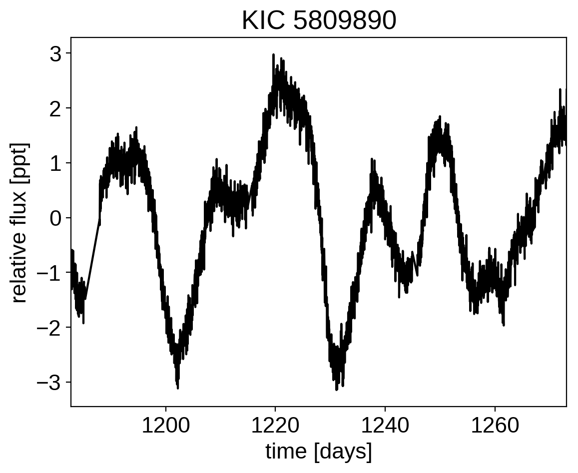
This looks like the light curve of a rotating star, and it has been shown that it is possible to model this variability by using a quasiperiodic Gaussian process. To start with, let’s get an estimate of the rotation period using the Lomb-Scargle periodogram:

import exoplanet as xo

results = xo.estimators.lomb_scargle_estimator(
    x, y, max_peaks=1, min_period=5.0, max_period=100.0, samples_per_peak=50
)

peak = results["peaks"][0]
freq, power = results["periodogram"]
plt.plot(1 / freq, power, "k")
plt.axvline(peak["period"], color="k", lw=4, alpha=0.3)
plt.xlim((1 / freq).min(), (1 / freq).max())
plt.yticks([])
plt.xlabel("period [days]")
plt.ylabel("power");

../../_images/stellar-variability_6_0.png

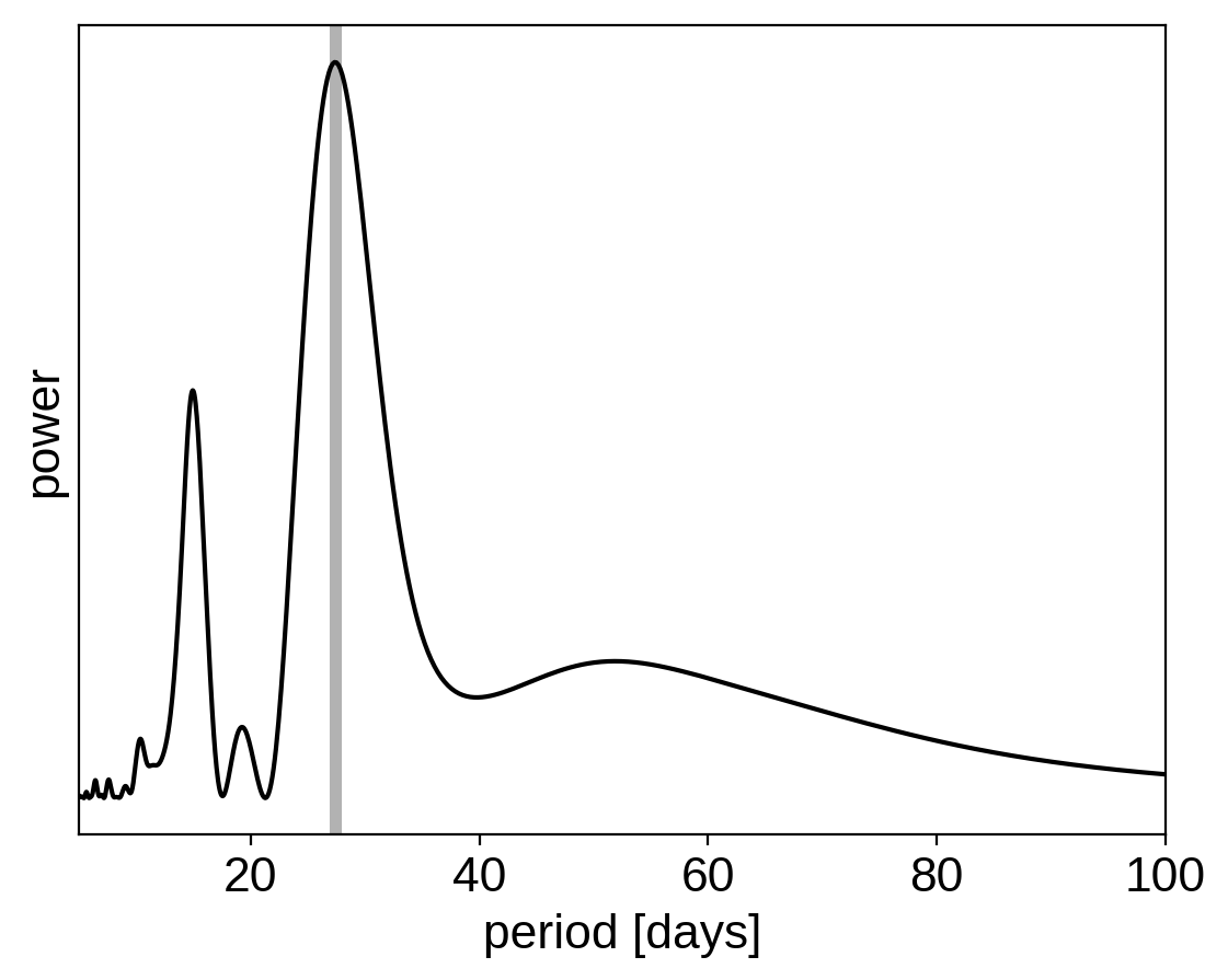
Now, using this initialization, we can set up the GP model in exoplanet. We’ll use the exoplanet.gp.terms.RotationTerm kernel that is a mixture of two simple harmonic oscillators with periods separated by a factor of two. As you can see from the periodogram above, this might be a good model for this light curve and I’ve found that it works well in many cases.

import pymc3 as pm
import theano.tensor as tt

with pm.Model() as model:

    # The mean flux of the time series
    mean = pm.Normal("mean", mu=0.0, sd=10.0)

    # A jitter term describing excess white noise
    logs2 = pm.Normal("logs2", mu=2 * np.log(np.mean(yerr)), sd=2.0)

    # A term to describe the non-periodic variability
    logSw4 = pm.Normal("logSw4", mu=np.log(np.var(y)), sd=5.0)
    logw0 = pm.Normal("logw0", mu=np.log(2 * np.pi / 10), sd=5.0)

    # The parameters of the RotationTerm kernel
    logamp = pm.Normal("logamp", mu=np.log(np.var(y)), sd=5.0)
    BoundedNormal = pm.Bound(pm.Normal, lower=0.0, upper=np.log(50))
    logperiod = BoundedNormal("logperiod", mu=np.log(peak["period"]), sd=5.0)
    logQ0 = pm.Normal("logQ0", mu=1.0, sd=10.0)
    logdeltaQ = pm.Normal("logdeltaQ", mu=2.0, sd=10.0)
    mix = xo.distributions.UnitUniform("mix")

    # Track the period as a deterministic
    period = pm.Deterministic("period", tt.exp(logperiod))

    # Set up the Gaussian Process model
    kernel = xo.gp.terms.SHOTerm(log_Sw4=logSw4, log_w0=logw0, Q=1 / np.sqrt(2))
    kernel += xo.gp.terms.RotationTerm(
        log_amp=logamp, period=period, log_Q0=logQ0, log_deltaQ=logdeltaQ, mix=mix
    )
    gp = xo.gp.GP(kernel, x, yerr ** 2 + tt.exp(logs2))

    # Compute the Gaussian Process likelihood and add it into the
    # the PyMC3 model as a "potential"
    pm.Potential("loglike", gp.log_likelihood(y - mean))

    # Compute the mean model prediction for plotting purposes
    pm.Deterministic("pred", gp.predict())

    # Optimize to find the maximum a posteriori parameters
    map_soln = xo.optimize(start=model.test_point)

optimizing logp for variables: [mix, logdeltaQ, logQ0, logperiod, logamp, logw0, logSw4, logs2, mean]
163it [00:11, 13.59it/s, logp=7.031724e+02]
message: Desired error not necessarily achieved due to precision loss.
logp: 267.25686032200514 -> 703.1723809089232

Now that we have the model set up, let’s plot the maximum a posteriori model prediction.

plt.plot(x, y, "k", label="data")
plt.plot(x, map_soln["pred"], color="C1", label="model")
plt.xlim(x.min(), x.max())
plt.legend(fontsize=10)
plt.xlabel("time [days]")
plt.ylabel("relative flux [ppt]")
plt.title("KIC 5809890; map model");

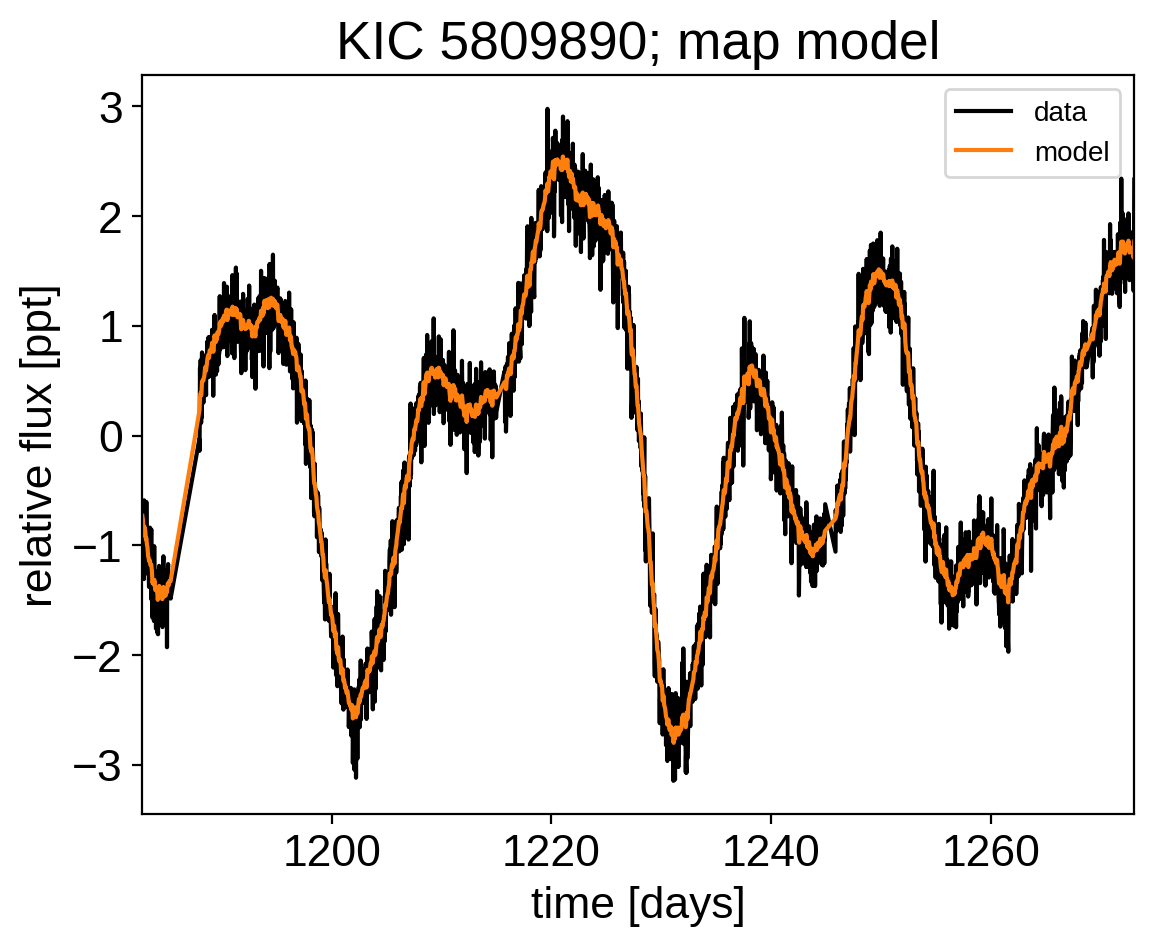
../../_images/stellar-variability_10_0.png

That looks pretty good! Now let’s sample from the posterior using exoplanet.get_dense_nuts_step().

np.random.seed(42)
with model:
    trace = pm.sample(
        tune=2000,
        draws=2000,
        start=map_soln,
        step=xo.get_dense_nuts_step(target_accept=0.9),
    )

Multiprocess sampling (4 chains in 4 jobs)
NUTS: [mix, logdeltaQ, logQ0, logperiod, logamp, logw0, logSw4, logs2, mean]
Sampling 4 chains: 100%|██████████| 16000/16000 [06:24<00:00, 41.60draws/s]
There were 2 divergences after tuning. Increase target_accept or reparameterize.
There were 2 divergences after tuning. Increase target_accept or reparameterize.
There were 5 divergences after tuning. Increase target_accept or reparameterize.
The number of effective samples is smaller than 25% for some parameters.

Now we can do the usual convergence checks:

pm.summary(
    trace,
    varnames=[
        "mix",
        "logdeltaQ",
        "logQ0",
        "logperiod",
        "logamp",
        "logSw4",
        "logw0",
        "logs2",
        "mean",
    ],
)

	mean	sd	mc_error	hpd_2.5	hpd_97.5	n_eff	Rhat
mix	0.638907	0.246249	0.005999	0.178848	0.999876	1388.904252	1.000946
logdeltaQ	0.622804	9.218069	0.181064	-17.817309	19.667857	2368.845797	1.000144
logQ0	0.781421	0.536186	0.007963	-0.247969	1.821605	3670.677635	0.999928
logperiod	3.326002	0.096711	0.002497	3.145160	3.528834	1366.843586	1.000468
logamp	0.384757	0.606889	0.013657	-0.588614	1.632578	1373.325178	1.000085
logSw4	6.610959	0.747819	0.012153	5.128654	8.023461	3602.498378	1.000397
logw0	3.861721	0.195403	0.002990	3.478037	4.236481	4046.885861	1.000415
logs2	-6.207327	0.682157	0.014721	-7.640965	-5.205967	2293.592072	1.000621
mean	-0.014214	0.202787	0.002961	-0.418842	0.384741	4635.502757	0.999902

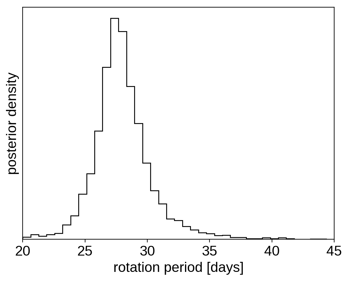
And plot the posterior distribution over rotation period:

period_samples = trace["period"]
bins = np.linspace(20, 45, 40)
plt.hist(period_samples, bins, histtype="step", color="k")
plt.yticks([])
plt.xlim(bins.min(), bins.max())
plt.xlabel("rotation period [days]")
plt.ylabel("posterior density");

../../_images/stellar-variability_16_0.png

Citations¶

As described in the Citing exoplanet & its dependencies tutorial, we can use exoplanet.citations.get_citations_for_model() to construct an acknowledgement and BibTeX listing that includes the relevant citations for this model.

with model:
    txt, bib = xo.citations.get_citations_for_model()
print(txt)

This research made use of textsf{exoplanet} citep{exoplanet} and its
dependencies citep{exoplanet:exoplanet, exoplanet:foremanmackey17,
exoplanet:foremanmackey18, exoplanet:pymc3, exoplanet:theano}.

print("\n".join(bib.splitlines()[:10]) + "\n...")

@misc{exoplanet:exoplanet,
  author = {Daniel Foreman-Mackey and Ian Czekala and Rodrigo Luger and
            Eric Agol and Geert Barentsen and Tom Barclay},
   title = {dfm/exoplanet: exoplanet v0.2.1},
   month = sep,
    year = 2019,
     doi = {10.5281/zenodo.3462740},
     url = {https://doi.org/10.5281/zenodo.3462740}
}
...

← Scalable Gaussian... Case study: K2-24, putting... →