Note
This tutorial was generated from an IPython notebook that can be downloaded here.
Fitting for or marginalizing over the transit times or transit timing
variations (TTVs) can be useful for several reasons, and it is a
compelling use case for exoplanet becuase the number of parameters
in the model increases significantly because there will be a new
parameter for each transit. The performance of the NUTS sampler used by
exoplanet scales well with the number of parameters, so a TTV model
should be substantially faster to run to convergence with exoplanet
than with other tools. There are a few definitions and subtleties that
should be considered before jumping in.
In this tutorial, we will be using a “descriptive” model
orbits.TTVOrbit to fit the light curve where the underlying
motion is still Keplerian, but the time coordinate is warped to make
t0 a function of time. All of the other orbital elements besides
t0 are shared across all orbits, but the t0 for each transit
will be a parameter. This means that other variations (like transit
duration variations) are not currently supported, but it would be
possible to include more general effects. exoplanet also supports
photodynamics modeling using the orbits.ReboundOrbit for more
detailed analysis, but that is a topic for a future tutorial.
It is also important to note that “transit time” within exoplanet
(and most other transit fitting software) is defined as the time of
conjunction (called t0 in the code): the time when the true anomaly
is \(\pi/2 - \omega\). Section 18 of the EXOFASTv2
paper includes an excellent
discussion of some of the commonly used definitions of “transit time” in
the literature.
Finally, there is a subtlety in the definition of the “period” of an
orbit with TTVs. Two possible definitions are: (1) the average time
between transits, or (2) the slope of a least squares fit to the transit
times as a function of transit number. In exoplanet, we use the
latter definition and call this parameter the ttv_period to
distinguish it from the period of the underlying Keplerian motion
which sets the shape and duration of the transit. By default, these two
periods are constrained to be equal, but it can be useful to fit for
both parameters since the shape of the transit might not be perfectly
described by the same period. That being said, if you fit for both
periods, make sure that you constrain ttv_period and period to
be similar or things can get a bit ugly.
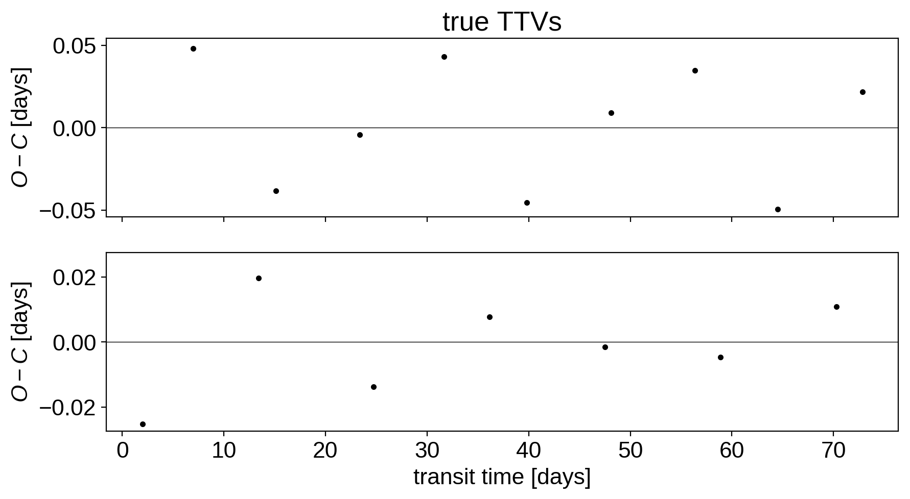
To get started, let’s generate some simulated transit times. We’ll use
the orbits.ttv.compute_expected_transit_times() function to get
the expected transit times for a linear ephemeris within some
observation baseline:
import numpy as np
import matplotlib.pyplot as plt

import exoplanet as xo

np.random.seed(3948)
true_periods = np.random.uniform(8, 12, 2)
true_t0s = true_periods * np.random.rand(2)
t = np.arange(0, 80, 0.01)
texp = 0.01
yerr = 5e-4

# Compute the transit times for a linear ephemeris
true_transit_times = xo.orbits.ttv.compute_expected_transit_times(
    t.min(), t.max(), true_periods, true_t0s
)

# Simulate transit timing variations using a simple model
true_ttvs = [
    (0.05 - (i % 2) * 0.1) * np.sin(2 * np.pi * tt / 23.7)
    for i, tt in enumerate(true_transit_times)
]
true_transit_times = [tt + v for tt, v in zip(true_transit_times, true_ttvs)]

# Plot the true TTV model
fig, (ax1, ax2) = plt.subplots(2, 1, figsize=(10, 5), sharex=True)
ax1.plot(true_transit_times[0], true_ttvs[0], ".k")
ax1.axhline(0, color="k", lw=0.5)
ax1.set_ylim(np.max(np.abs(ax1.get_ylim())) * np.array([-1, 1]))
ax1.set_ylabel("$O-C$ [days]")

ax2.plot(true_transit_times[1], true_ttvs[1], ".k")
ax2.axhline(0, color="k", lw=0.5)
ax2.set_ylim(np.max(np.abs(ax2.get_ylim())) * np.array([-1, 1]))
ax2.set_ylabel("$O-C$ [days]")

ax2.set_xlabel("transit time [days]")
ax1.set_title("true TTVs");
Now, like in the Transit fitting tutorial, we’ll set up the the model
using PyMC3 and exoplanet, and then simulate a data set from
that model.
import pymc3 as pm
import theano.tensor as tt

np.random.seed(9485023)

with pm.Model() as model:

    # This part of the model is similar to the model in the `transit` tutorial
    mean = pm.Normal("mean", mu=0.0, sd=1.0)
    u = xo.distributions.QuadLimbDark("u", testval=np.array([0.3, 0.2]))
    logr = pm.Uniform(
        "logr",
        lower=np.log(0.01),
        upper=np.log(0.1),
        shape=2,
        testval=np.log([0.04, 0.06]),
    )
    r = pm.Deterministic("r", tt.exp(logr))
    b = xo.distributions.ImpactParameter(
        "b", ror=r, shape=2, testval=0.5 * np.random.rand(2)
    )

    # Now we have a parameter for each transit time for each planet:
    transit_times = []
    for i in range(2):
        transit_times.append(
            pm.Normal(
                "tts_{0}".format(i),
                mu=true_transit_times[i],
                sd=1.0,
                shape=len(true_transit_times[i]),
            )
        )

    # Set up an orbit for the planets
    orbit = xo.orbits.TTVOrbit(b=b, transit_times=transit_times)

    # It will be useful later to track some parameters of the orbit
    pm.Deterministic("t0", orbit.t0)
    pm.Deterministic("period", orbit.period)
    for i in range(2):
        pm.Deterministic("ttvs_{0}".format(i), orbit.ttvs[i])

    # The rest of this block follows the transit fitting tutorial
    light_curves = xo.LimbDarkLightCurve(u).get_light_curve(
        orbit=orbit, r=r, t=t, texp=texp
    )
    light_curve = pm.math.sum(light_curves, axis=-1) + mean
    pm.Deterministic("light_curves", light_curves)
    y = xo.eval_in_model(light_curve)
    y += yerr * np.random.randn(len(y))
    pm.Normal("obs", mu=light_curve, sd=yerr, observed=y)

    map_soln = model.test_point
    map_soln = xo.optimize(start=map_soln, vars=transit_times)
    map_soln = xo.optimize(start=map_soln, vars=[r, b])
    map_soln = xo.optimize(start=map_soln, vars=transit_times)
    map_soln = xo.optimize(start=map_soln)
optimizing logp for variables: [tts_1, tts_0]
120it [00:04, 26.01it/s, logp=4.946128e+04]
message: Desired error not necessarily achieved due to precision loss.
logp: 49454.87884962603 -> 49461.28172640355
optimizing logp for variables: [b, logr]
18it [00:00, 23.53it/s, logp=4.946356e+04]
message: Optimization terminated successfully.
logp: 49461.28172640355 -> 49463.56218609357
optimizing logp for variables: [tts_1, tts_0]
53it [00:01, 48.16it/s, logp=4.946363e+04]
message: Desired error not necessarily achieved due to precision loss.
logp: 49463.56218609357 -> 49463.626773189084
optimizing logp for variables: [tts_1, tts_0, b, logr, u, mean]
113it [00:01, 88.99it/s, logp=4.946400e+04]
message: Desired error not necessarily achieved due to precision loss.
logp: 49463.626773189084 -> 49464.004718781114
Here’s our simulated light curve and the initial model:
plt.plot(t, y, ".k", ms=4, label="data")
for i, l in enumerate("bc"):
    plt.plot(t, map_soln["light_curves"][:, i], lw=1, label="planet {0}".format(l))
plt.xlim(t.min(), t.max())
plt.ylabel("relative flux")
plt.xlabel("time [days]")
plt.legend(fontsize=10)
plt.title("map model");
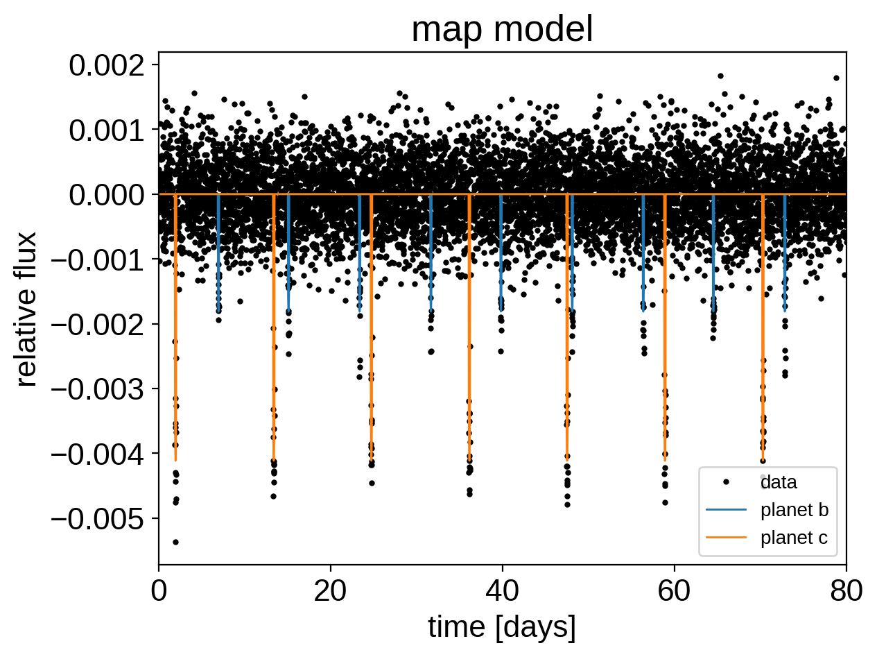
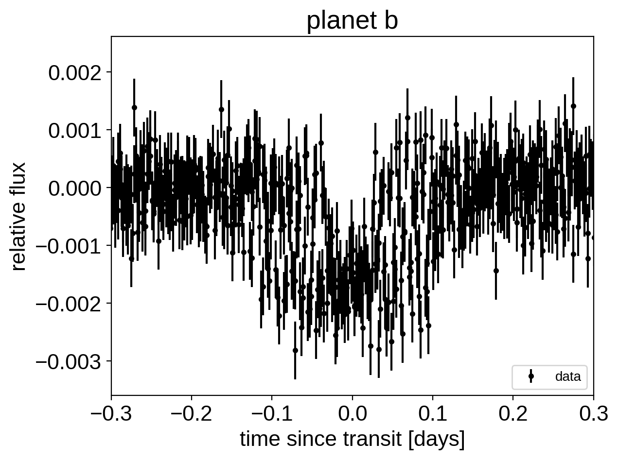
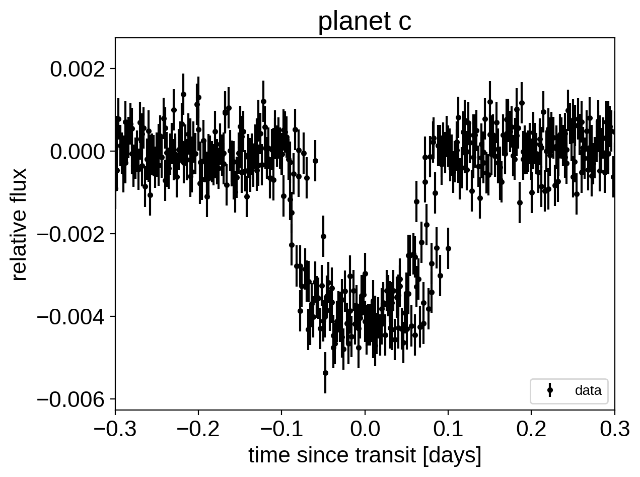
This looks similar to the light curve from the Transit fitting tutorial, but if we try plotting the folded transits, we can see that something isn’t right: these transits look pretty smeared out!
for n, letter in enumerate("bc"):
    plt.figure()

    # Get the posterior median orbital parameters
    p = map_soln["period"][n]
    t0 = map_soln["t0"][n]

    # Compute the median of posterior estimate of the contribution from
    # the other planet. Then we can remove this from the data to plot
    # just the planet we care about.
    other = map_soln["light_curves"][:, (n + 1) % 2]

    # Plot the folded data
    x_fold = (t - t0 + 0.5 * p) % p - 0.5 * p
    plt.errorbar(x_fold, y - other, yerr=yerr, fmt=".k", label="data", zorder=-1000)

    plt.legend(fontsize=10, loc=4)
    plt.xlim(-0.5 * p, 0.5 * p)
    plt.xlabel("time since transit [days]")
    plt.ylabel("relative flux")
    plt.title("planet {0}".format(letter))
    plt.xlim(-0.3, 0.3)
Instead, we can correct for the transit times by removing the best fit transit times and plot that instead:
with model:
    t_warp = xo.eval_in_model(orbit._warp_times(t), map_soln)

for n, letter in enumerate("bc"):
    plt.figure()

    p = map_soln["period"][n]
    other = map_soln["light_curves"][:, (n + 1) % 2]

    # NOTE: 't0' has already been subtracted!
    x_fold = (t_warp[:, n] + 0.5 * p) % p - 0.5 * p
    plt.errorbar(x_fold, y - other, yerr=yerr, fmt=".k", label="data", zorder=-1000)

    plt.legend(fontsize=10, loc=4)
    plt.xlim(-0.5 * p, 0.5 * p)
    plt.xlabel("time since transit [days]")
    plt.ylabel("relative flux")
    plt.title("planet {0}".format(letter))
    plt.xlim(-0.3, 0.3)
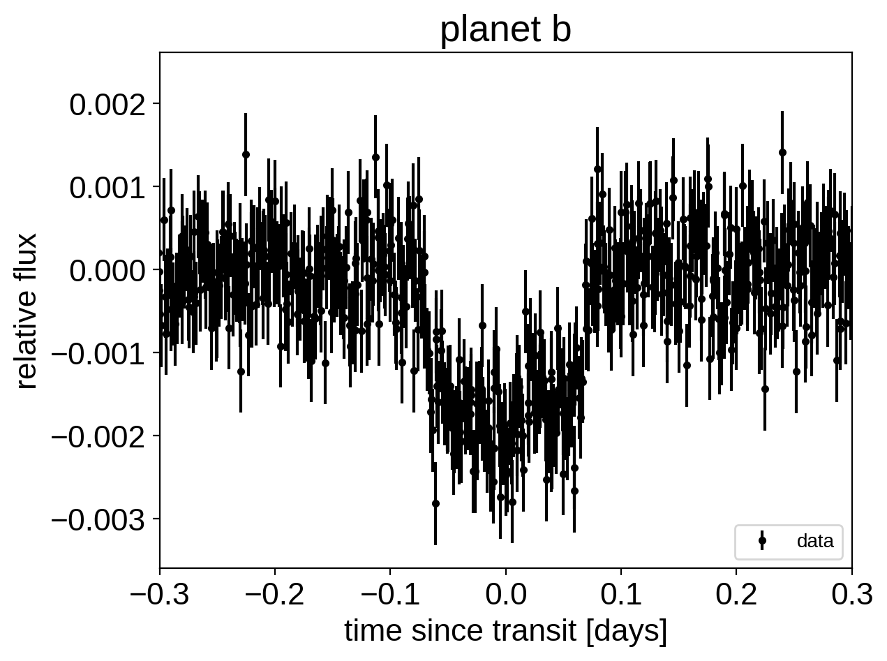
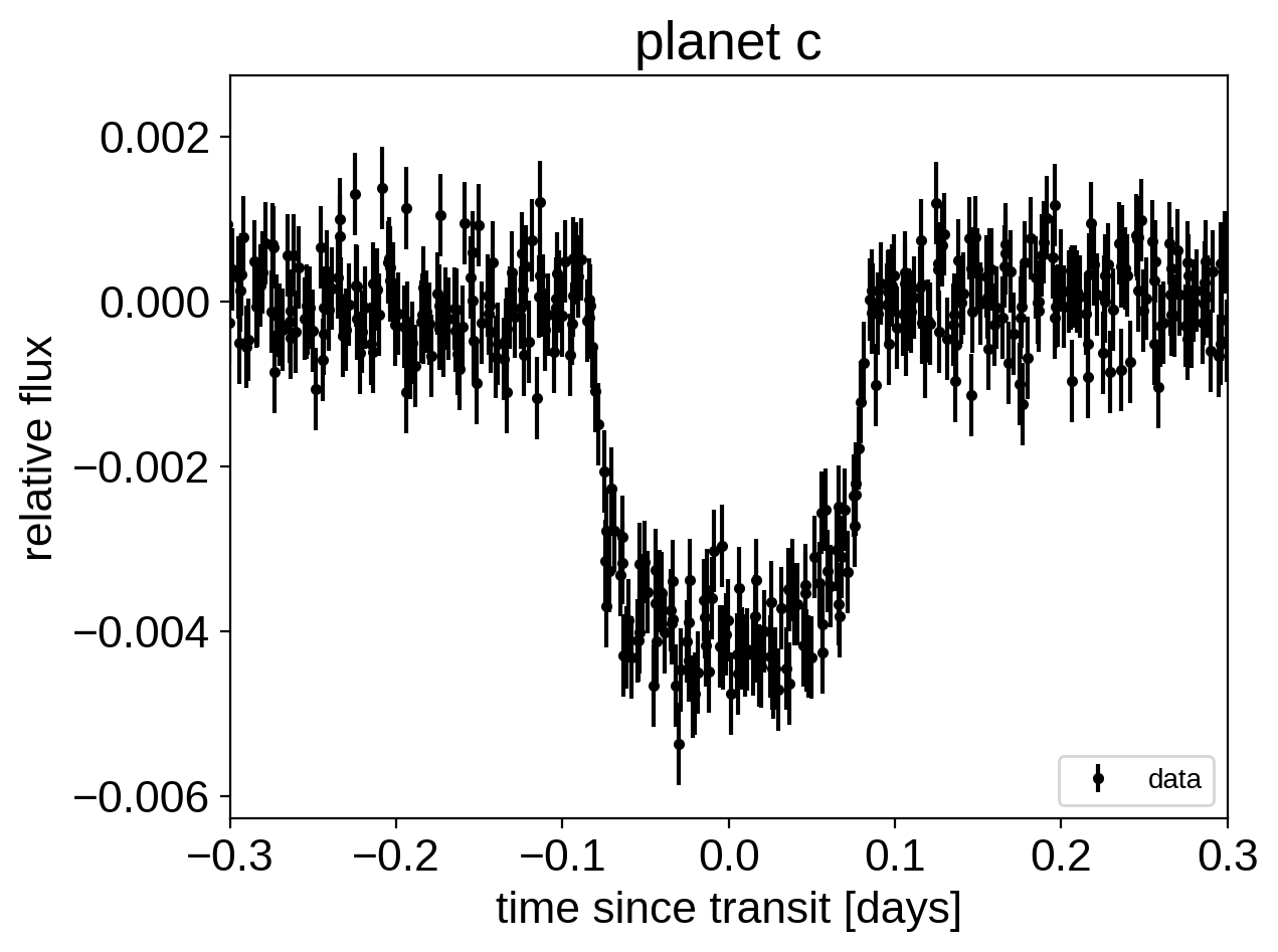
That looks better!
Now let’s run some MCMC as usual:
np.random.seed(230948)
with model:
    trace = pm.sample(
        tune=1000,
        draws=1000,
        start=map_soln,
        step=xo.get_dense_nuts_step(target_accept=0.9),
    )
Multiprocess sampling (4 chains in 4 jobs)
NUTS: [tts_1, tts_0, b, logr, u, mean]
Sampling 4 chains: 100%|██████████| 8000/8000 [01:52<00:00, 71.38draws/s]
Then check the convergence diagnostics:
pm.summary(trace, varnames=["mean", "u", "logr", "b", "tts_0", "tts_1"])
| mean | sd | mc_error | hpd_2.5 | hpd_97.5 | n_eff | Rhat | |
|---|---|---|---|---|---|---|---|
| mean | -0.000003 | 0.000006 | 6.036550e-08 | -0.000014 | 0.000008 | 7951.264445 | 0.999598 |
| u__0 | 0.342717 | 0.171603 | 3.127874e-03 | 0.012857 | 0.625676 | 3307.235257 | 0.999786 |
| u__1 | 0.178007 | 0.297945 | 5.648345e-03 | -0.324534 | 0.719815 | 2888.604157 | 0.999622 |
| logr__0 | -3.222882 | 0.019438 | 3.078609e-04 | -3.261813 | -3.186574 | 3630.177143 | 0.999938 |
| logr__1 | -2.813157 | 0.012714 | 2.314427e-04 | -2.839966 | -2.790918 | 2983.225881 | 0.999739 |
| b__0 | 0.394382 | 0.043633 | 8.273671e-04 | 0.305350 | 0.473317 | 2841.660084 | 1.000083 |
| b__1 | 0.354436 | 0.030505 | 5.763580e-04 | 0.293155 | 0.408723 | 2606.185780 | 0.999798 |
| tts_0__0 | 6.962988 | 0.004645 | 7.883311e-05 | 6.954894 | 6.972102 | 3957.707556 | 1.000532 |
| tts_0__1 | 15.105173 | 0.006857 | 1.375224e-04 | 15.091271 | 15.116490 | 2590.207778 | 1.000638 |
| tts_0__2 | 23.380438 | 0.002205 | 2.809419e-05 | 23.376013 | 23.384614 | 5843.603039 | 0.999822 |
| tts_0__3 | 31.666856 | 0.003857 | 4.944050e-05 | 31.659030 | 31.673703 | 6286.150816 | 0.999847 |
| tts_0__4 | 39.813239 | 0.002718 | 3.407893e-05 | 39.808318 | 39.818873 | 6735.112313 | 0.999776 |
| tts_0__5 | 48.105357 | 0.003237 | 4.216364e-05 | 48.099165 | 48.111476 | 6479.282957 | 0.999918 |
| tts_0__6 | 56.371431 | 0.003099 | 4.131000e-05 | 56.365803 | 56.378123 | 5316.468567 | 0.999730 |
| tts_0__7 | 64.525313 | 0.001875 | 2.405386e-05 | 64.521625 | 64.528931 | 7065.382141 | 1.000028 |
| tts_0__8 | 72.834911 | 0.002607 | 3.131700e-05 | 72.829892 | 72.840116 | 7760.060791 | 0.999530 |
| tts_1__0 | 1.970518 | 0.001536 | 1.936021e-05 | 1.967514 | 1.973597 | 6230.401871 | 0.999885 |
| tts_1__1 | 13.395061 | 0.001442 | 1.642121e-05 | 13.392272 | 13.397960 | 7184.991129 | 0.999723 |
| tts_1__2 | 24.743927 | 0.001394 | 1.624029e-05 | 24.741089 | 24.746494 | 7539.455329 | 0.999579 |
| tts_1__3 | 36.143523 | 0.001219 | 1.501228e-05 | 36.141029 | 36.145809 | 7086.565692 | 0.999945 |
| tts_1__4 | 47.512046 | 0.001427 | 1.718606e-05 | 47.509357 | 47.514923 | 8361.206162 | 1.000228 |
| tts_1__5 | 58.888722 | 0.001301 | 1.681865e-05 | 58.886356 | 58.891440 | 6284.273858 | 1.000194 |
| tts_1__6 | 70.284253 | 0.001227 | 1.386730e-05 | 70.281896 | 70.286663 | 6423.395074 | 0.999581 |
And plot the corner plot of the physical parameters:
import corner

with model:
    truths = np.concatenate(
        list(map(np.atleast_1d, xo.eval_in_model([orbit.period, r, b])))
    )
samples = pm.trace_to_dataframe(trace, varnames=["period", "r", "b"])
corner.corner(
    samples,
    truths=truths,
    labels=["period 1", "period 2", "radius 1", "radius 2", "impact 1", "impact 2"],
);
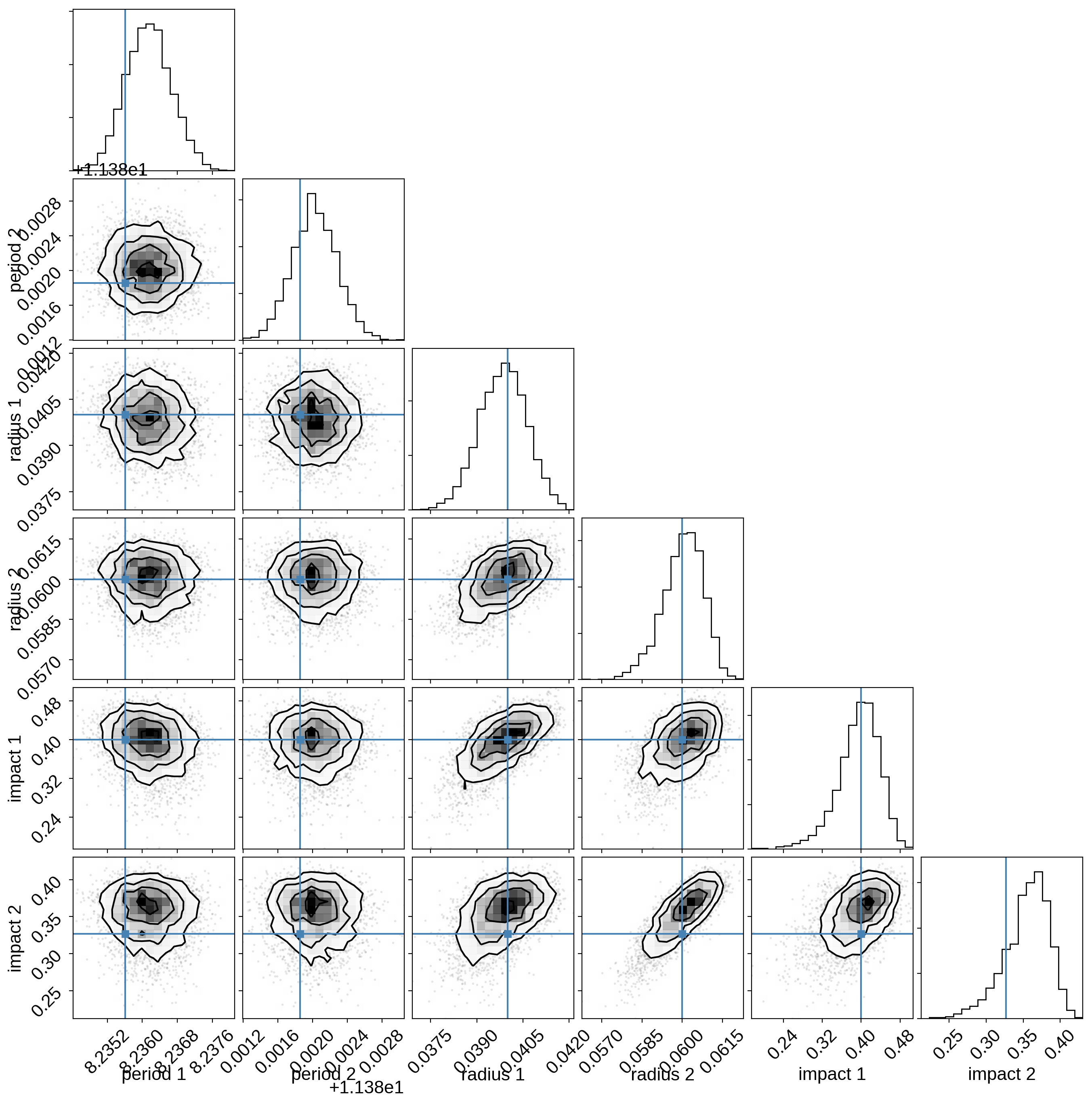
We could also plot corner plots of the transit times, but they’re not terribly enlightening in this case so let’s skip it.
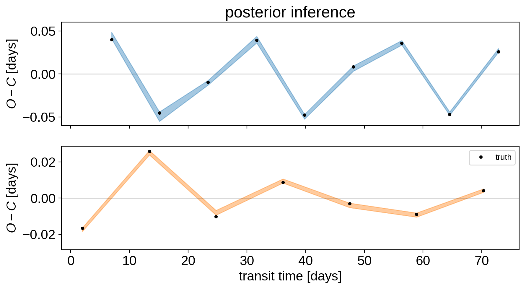
Finally, let’s plot the posterior estimates of the the transit times in an O-C diagram:
fig, (ax1, ax2) = plt.subplots(2, 1, figsize=(10, 5), sharex=True)

q = np.percentile(trace["ttvs_0"], [16, 50, 84], axis=0)
ax1.fill_between(
    np.mean(trace["tts_0"], axis=0), q[0], q[2], color="C0", alpha=0.4, edgecolor="none"
)
ref = np.polyval(
    np.polyfit(true_transit_times[0], true_ttvs[0], 1), true_transit_times[0]
)
ax1.plot(true_transit_times[0], true_ttvs[0] - ref, ".k")
ax1.axhline(0, color="k", lw=0.5)
ax1.set_ylim(np.max(np.abs(ax1.get_ylim())) * np.array([-1, 1]))

ax1.set_ylabel("$O-C$ [days]")

q = np.percentile(trace["ttvs_1"], [16, 50, 84], axis=0)
ax2.fill_between(
    np.mean(trace["tts_1"], axis=0), q[0], q[2], color="C1", alpha=0.4, edgecolor="none"
)
ref = np.polyval(
    np.polyfit(true_transit_times[1], true_ttvs[1], 1), true_transit_times[1]
)
ax2.plot(true_transit_times[1], true_ttvs[1] - ref, ".k", label="truth")
ax2.axhline(0, color="k", lw=0.5)
ax2.set_ylim(np.max(np.abs(ax2.get_ylim())) * np.array([-1, 1]))

ax2.legend(fontsize=10)
ax2.set_ylabel("$O-C$ [days]")
ax2.set_xlabel("transit time [days]")
ax1.set_title("posterior inference");
As described in the Citing exoplanet & its dependencies tutorial, we can use
exoplanet.citations.get_citations_for_model() to construct an
acknowledgement and BibTeX listing that includes the relevant citations
for this model.
with model:
    txt, bib = xo.citations.get_citations_for_model()
print(txt)
This research made use of textsf{exoplanet} citep{exoplanet} and its
dependencies citep{exoplanet:agol19, exoplanet:astropy13, exoplanet:astropy18,
exoplanet:exoplanet, exoplanet:kipping13, exoplanet:luger18, exoplanet:pymc3,
exoplanet:theano}.
print("\n".join(bib.splitlines()[:10]) + "\n...")
@misc{exoplanet:exoplanet,
  author = {Daniel Foreman-Mackey and Ian Czekala and Rodrigo Luger and
            Eric Agol and Geert Barentsen and Tom Barclay},
   title = {dfm/exoplanet},
   month = sep,
    year = 2019,
     doi = {10.5281/zenodo.1998447},
     url = {https://doi.org/10.5281/zenodo.1998447}
}
...